Global Alignment Problem

The solution to the Manhattan problem described here only returned us the maximum score, but did not give instructions on how exactly we should walk through Manhattan to achieve this score. To lay out the path (and to use the solution in bioinformatics to align aminoacid sequences) we need an additional step: keep the history of our walk so that we could "backtrack" from the last intersection all the way back to the start. Essentially, it is simple: when we arrive to a new node, we always come from somewhere. This is the node we need to remember.

We should also consider that, unlike Manhattan graph, where we only had streets going "west" or "south", we now have "diagonal" streets if we want to adapt the problem to align aminoacid sequences. Consider the image below:

Alignment graph matches

The red diagonal arrows show the places where one sequence matches the other. We can give these edges a higher "score" so the path that goes through most of such edges is the highest scored. In this case we have three ways to reach any node s[i,j]: we can come from s[i - 1,j] by moving down, from s[i,j - 1] by moving right, or from s[i - 1, j - 1] by moving diagonally. In the simplest case, we'll calculate anything other than a match as a 0, and a match as 1. Then the score for any s[i,j] node will be calculated using the following formula:

Global alignment formula

In more complex scenarios, we may use scoring matrices, where each combination of two aminoacids is given a certain score, depending on how biologically reasonable is this combination.

Therefore, the following algorithm is used to calculate the score matrix s, and at the same time fill the backtracking matrix backtrack.

AlignmentMatrix(v, w)
 for i ← 0 to |v|
  si, 0 ← 0
 for j ← 0 to |w| 
  s0, j ← 0
 for i ← 1 to |v|
  for j ← 1 to |w|
   si, j = max{si-1, j, si,j-1, si-1, j-1 + 1 (if vi = wj)}
   backtracki, j = ↓ if si, j = si-1, j ; → if si, j = si, j-1 ; ↘ if si, j = si-1, j-1 + 1
 return s|v|, |w| , backtrack

After both the scoring matrices are filled, we will use the following algorithm to backtrack from the s[i,j] all the way back to the starting node. Along the way we will output two string. In places where there is a match between the strings, a symbol will be placed, and in other places we will fill in a dash. Following is the backtracking algorithm. We are filling two strings, v and w. If we came to the point i,j by a diagonal edge, we have a match, and output the same symbol into both strings. If we came by a vertical or horisontal edge, one of the strings receives a symbol, and the other a "mismatch" - a "-".

OUTPUTALIGNMENT(backtrack, v, w, i, j)
 if i = 0 or j = 0
  return
 if backtracki, j = ↓
  output vi = "-"
  outpuv wi
  OUTPUTLCS(backtrack, v, i - 1, j)
 else if backtracki, j = →
  output vi
  output wi = "-"
  OUTPUTLCS(backtrack, v, i, j - 1)
 else
  OUTPUTLCS(backtrack, v, i - 1, j - 1)
  output vi
  output wi

This is the C# implementation of the algorithms.

public static void GlobalAlignment(string s1, string s2)
{
 int s1l = s1.Length;
 int s2l = s2.Length;

 int[,] matrix = new int[s1l + 1, s2l + 1];
 int[,] backtrack = new int[s1l + 1, s2l + 1];

 for (int i = 0; i <= s1l; i++) for (int j = 0; j <= s2l; j++) matrix[i, j] = 0;
 for (int i = 0; i <= s1l; i++) for (int j = 0; j <= s2l; j++) backtrack[i, j] = 0;

 for (int i = 0; i <= s1l; i++) matrix[i, 0] = 0;
 for (int j = 0; j <= s2l; j++) matrix[0, j] = 0;

 for (int i = 1; i <= s1l; i++)
 {
  for (int j = 1; j <= s2l; j++)
  {
   matrix[i, j] = Math.Max(Math.Max(matrix[i - 1, j], matrix[i, j - 1]), matrix[i - 1, j - 1] + 1);

   if (matrix[i, j] == matrix[i - 1, j]) backtrack[i, j] = -1;
   else if (matrix[i, j] == matrix[i, j - 1]) backtrack[i, j] = -2;
   else if (matrix[i, j] == matrix[i - 1, j - 1] + 1) backtrack[i, j] = 1;
  }
 }

 OUTPUTLCSALIGN(backtrack, s2, s1, s1l, s2l);

 string aligned1 = ReverseString(Result);
 string aligned2 = ReverseString(Result2);
}

public static void OUTPUTLCSALIGN(int[,] backtrack, string v, string w, int i, int j)
{
 if (i == 0 || j == 0)
  return;
 if (backtrack[i, j] == -1)
 {
  Result = Result + "-";
  Result2 = Result2 + w[i - 1];
  OUTPUTLCSALIGN(backtrack, v, w, i - 1, j);
 }
 else if (backtrack[i, j] == -2)
 {
  Result = Result + v[j - 1];
  Result2 = Result2 + "-";
  OUTPUTLCSALIGN(backtrack, v, w, i, j - 1);
 }
 else
 {
  Result = Result + v[j - 1];
  Result2 = Result2 + w[i - 1];
  OUTPUTLCSALIGN(backtrack, v, w, i - 1, j - 1);
 }
}

public static string ReverseString(string input)
{
 char[] charArray = input.ToCharArray();
 Array.Reverse(charArray);
 return new string(charArray);
}

A slightly modified version of the function takes into account a penalty for an insertion / deletion (-5 in this case) and uses a BLOSUM62 scoring matrix

public static void GlobalAlignment(string s1, string s2)
{
 int indelPenalty = -5;

 int s1l = s1.Length;
 int s2l = s2.Length;

 int[,] matrix = new int[s1l + 1, s2l + 1];
 int[,] backtrack = new int[s1l + 1, s2l + 1];

 for (int i = 0; i <= s1l; i++) for (int j = 0; j <= s2l; j++) matrix[i, j] = 0;
 for (int i = 0; i <= s1l; i++) for (int j = 0; j <= s2l; j++) backtrack[i, j] = 0;

 for (int i = 0; i <= s1l; i++) matrix[i, 0] = indelPenalty * i;
 for (int j = 0; j <= s2l; j++) matrix[0, j] = indelPenalty * j;

 for (int i = 1; i <= s1l; i++)
 {
  for (int j = 1; j <= s2l; j++)
  {
   //deletion
   int delCoef = matrix[i - 1, j] + indelPenalty;
   //insertion
   int insCoef = matrix[i, j - 1] + indelPenalty;
   //match / mismatch
   int mCoef = matrix[i - 1, j - 1] + BlosumCoeff(s1[i - 1], s2[j - 1]);

   matrix[i, j] = Math.Max(Math.Max(delCoef, insCoef), mCoef);

   if (matrix[i, j] == delCoef) backtrack[i, j] = -1; //
   else if (matrix[i, j] == insCoef) backtrack[i, j] = -2; //
   else if (matrix[i, j] == mCoef) backtrack[i, j] = 1;
  }
 }

 OUTPUTLCSALIGN(backtrack, s2, s1, s1l, s2l);

 string aligned1 = ReverseString(Result);
 string aligned2 = ReverseString(Result2);
}

Given the following two strings

PLEASANTLY
MEANLY

The following alignment will be returned

PLEASANTLY
-MEA--N-LY

by Evgeny. Also posted on my website

Manhattan Tourist Problem

An introductory exercise to aligning amino acid sequences is the Manhattan tourist problem. Suppose a tourist starts his route in the top left corner of the map and wants to visit as many attractions on the way as possible, and finish in the down right corner. There is a restriction however - he can only move either to the right or down.

A Simplified Map of Manhattan

To describe the problem in numbers and data structures, the map is converted to the directed grid shown below. A tourist can move along the edges of the grid and the score of 1 is added if he passes an attraction, which are assigned to the bold edges. Of all possible paths we are interested in the one with the highest score.

Map of Manhattan as a Graph

The solution to this problem is equivalent to a more general problem. This time every "street", or the edge of the graph, is assigned a score. The goal is to find a path which gains the highest score.

Generic Manhattan Problem

The problem can be brute forced, of course, by calculating the score for all possible paths. This is not practical for the larger graphs of course. A better approach is to calculate the highest possible score at every intersection, starting from the top left corner. Here is how the logic goes: If the tourist goes only towards the left in the grid, or only down, there are no choices for him. So it is easy to calculate the highest scores for the top and left row of intersections. Now we have these scores calculated:

Generic Manhattan Problem - First Row and Column Solved

Now when that's done, we can proceed to the next row. How can the tourist get to intersection (1, 1)? He can either go to (0, 1) first, and gain 3 + 0 = 3 score, or go to (1, 0) and gain 1 + 3 = 4 score. Therefore, the maximum score he can gain at (1, 1) is 4.

Generic Manhattan Problem - Cell (1,1) Solved

The generic formula to use is quite intuitive: To reach an intersection, you have to arrive from one of two possible previous locations, and traverse a corresponding edge. You choose the path where the sum of the score of a previous location, plus the score of the edge, is higher.

Generic Manhattan Formula

We continue calculations along the column all the way down. After that, we can move on to the next row.

Generic Manhattan Problem - Second Column Solved

Following this logic, it is easy to compute the maximum score for each intersection and find out the maximum score that can be gained while traversing Manhattan.

Generic Manhattan Problem - Fully Solved

Along the way the algorithm also becomes clear: the maximum score at any intersection is the maximum of the following two values:

MANHATTANTOURIST(n, m, down, right)
 s0, 0 ← 0
 for i ← 1 to n
  si, 0 ← si-1, 0 + downi, 0
 for j ← 1 to m
  s0, j ← s0, j−1 + right0, j
 for i ← 1 to n
  for j ← 1 to m
   si, j ← max{si - 1, j + downi, j, si, j - 1 + righti, j}
 return sn, m

The following C# function implements the algorithm and returns the highest possible score, assuming we input all the scores for the edges towards the right and all the edges pointing down in the form of two-dimension arrays.

public static int ManhattanProblem(int[,] RightMatrix, int[,] DownMatrix)
{
 int n = RightMatrix.GetLength(0) + 1;
 int m = DownMatrix.GetLength(1) + 1;
 int[,] ManhattanMatrix = new int[n, m];

 ManhattanMatrix[0, 0] = 0;

 for (int i = 1; i <= n; i++)
 {
  ManhattanMatrix[i, 0] = ManhattanMatrix[i - 1, 0] + DownMatrix[i - 1, 0];
 }

 for (int j = 1; j <= m; j++)
 {
  ManhattanMatrix[0, j] = ManhattanMatrix[0, j - 1] + RightMatrix[0, j - 1];
 }

 for (int i = 1; i <= n; i++)
 {
  for (int j = 1; j <= m; j++)
  {
   ManhattanMatrix[i, j] =
    Math.Max(ManhattanMatrix[i - 1, j] + DownMatrix[i - 1, j], 
    ManhattanMatrix[i, j - 1] + RightMatrix[i, j - 1]);
  }
 }

 return ManhattanMatrix.Cast<int>().Max();
}

Understanding this problem turns out to be important to understanding sequence alignment in bioinformatics.

by Evgeny. Also posted on my website

Stochastic and deterministic modelling.

Stochastic and deterministic modelling.

1. Purposes of stochastic modelling

Deterministic modelling assumes the systems to be continuous and evolve deterministically. The behaviour of the system can be described using ODEs, which are then solved. However, such models ignore the phenomena that occur due to the fact that each system consists of a finite number of discrete particles, such as random fluctuations. For systems with very small particle numbers the deterministic models are not even appropriate because the concentrations are not continuous.

Stochastic modelling takes into account the fact that each system is composed of a finite and countable number of particles and considers the number of those particles similar to the way the deterministic system considers concentrations.

2. Drawbacks of stochastic modelling

2.1. Limits on particle numbers

Considering the fact that the number of particles in the system is very large, computational modelling of a stochastic method is very demanding and developing an algorithm is a complex task.

2.2. Lack of analysis methods

Stochastic modelling does not have such rigorously developed analysis methods as metabolic control analysis for deterministic modelling.

3. Drawbacks of deterministic modelling

3.1. Systems with small particle numbers

Stochastic methods consider random fluctuations which lead to significant change in system behaviour when the number of particles is small. Species are allowed to become extinct. In deterministic models the fluctuations are not accounted for and species concentrations never fall to zero. Therefore, in linear processes, the deterministic model behaviour will only be determined by difference in concentrations. The stochastic models can behave differently. This remains true even if stochastic systems have the same marginal distribution of system states.

3.2. Bi-Stable systems

Under deterministic simulation the system which is bi-stable will converge to the same stable steady state if the initial concentrations remain the same. Under stochastic simulation the system will converge to one of the two stable states, and it can not be predicted to which one. The probability of the system converging to each state, however, can be calculated.

4. Difference between the deterministic solution and the mean of stochastic solutions

It should be noted that if we repeat the stochastic simulation many times and calculate the mean, we will not end up with the same solution as the deterministic. This is only true for linear systems, but the solutions for nonlinear systems can be totally different.

5. Conclusion

Stochastic modelling should definitely be chosen when the particle numbers are in range where the concept of continuous concentration is no longer applicable or when the stochastic phenomena are themselves the object of research. The limit on the application of stochastic model is generally enforced at a certain particle number where computation becomes not feasible.

References

Pahle J, Biochemical simulations: stochastic, approximate stochastic and hybrid approaches, Briefings in Bioinformatics 2009, 10(1), pp 53-64

by Evgeny. Also posted on my website

Project ROSALIND: Finding a shortest superstring

For a collection of strings, a larger string containing every one of the smaller strings as a substring is called a superstring. This may be useful, for example, if we have a large number of pieces of a DNA and want to figure out how the full DNA could look like.

For example, for the following strings

ATTAGACCTG
CCTGCCGGAA
AGACCTGCCG
GCCGGAATAC

The shortest superstring will be

ATTAGACCTGCCGGAATAC

The following code is a naive approach to solve the problem. The logic is as follows: Sort the list of strings by length. Take the longest one and call it a superstring. Next, iterate through the list to find the string that has the longest intersection with the superstring. Remove that string from the list and attach to the superstring. Continue until the list is empty, the resulting superstring should be the shortest possible.

public static string ShortestSuperstring(List<string> input)
{
 input = input.OrderByDescending(x => x.Length).ToList();

 string superstring = input[0];
 input.RemoveAt(0);
 int counter = input.Count;
 for (int i = 0; i < counter; i++)
 {
  List<IntBoolString> items = new List<IntBoolString>();

  for (int j = 0; j < input.Count; j++)
  {
   items.Add(GetIntersection(superstring, input[j]));
  }

  IntBoolString chosen = items.OrderByDescending(x => x.intValue).First();

  superstring = CombineIntoSuper(superstring, chosen);
  input.Remove(chosen.stringValue);
 }

 return superstring;
}

private static IntBoolString GetIntersection(string super, string candidate)
{
 IntBoolString result = new IntBoolString();
 result.stringValue = candidate;

 int i = 0;

 while (candidate.Length > i)
 {
  int testlen = candidate.Length - i;
  string leftcan = candidate.Substring(0, testlen);
  string rightcan = candidate.Substring(i, testlen);
  string leftsuper = super.Substring(0, testlen);
  string rightsuper = super.Substring(super.Length - testlen, testlen);

  if (leftcan == rightsuper || rightcan == leftsuper)
  {
   result.boolValue = (leftcan == rightsuper) ? true : false;
   result.intValue = testlen;
   return result;
  }

  i++;
 }

 return result;
}

private static string CombineIntoSuper(string superstring, IntBoolString chosen)
{
 string toAppend = string.Empty;
 int lenToAppend = chosen.stringValue.Length - chosen.intValue;

 toAppend = (chosen.boolValue == true) ?
  chosen.stringValue.Substring(chosen.stringValue.Length - lenToAppend, lenToAppend) :
  chosen.stringValue.Substring(0, lenToAppend);

 superstring = (chosen.boolValue == true) ?
  superstring + toAppend :
  toAppend + superstring;

 return superstring;
}

public struct IntBoolString
{
 public string stringValue;
 public int intValue;
 public bool boolValue;
}

by Evgeny. Also posted on my website

Some string manipulations for future use.

1. Using an array of characters, return all possible permutations of this array (without repetitions).

public static List<string> StringPermutations(char[] list)
{
 List<string> result = new List<string>();
 int x=list.Length-1;
 go(list,0,x, result);
 return result;
}

private static void go (char[] list, int k, int m, List<string> result)
{
 int i;
 if (k == m)
 {
  result.Add(new string(list));
 }
 else
 for (i = k; i <= m; i++)
 {
  swap (ref list[k],ref list[i]);
  go (list, k+1, m, result);
  swap (ref list[k],ref list[i]);
 }
}

private static void swap(ref char a, ref char b)
{
 if (a == b) return;
 a ^= b;
 b ^= a;
 a ^= b;
}

Sample usage

List<string> permutations = Helper.StringPermutations(new char[] {'D', 'N', 'A'});

Sample output

DNA
DAN
NDA
NAD
AND
ADN

2. Using an array of characters ("alphabet"), return all possible words generated from this alphabet of a specified length

public static IEnumerable<String> GetWordsWithRepetition(Int32 length, char[] alphabet)
{
 if (length <= 0)
  yield break;

 for(int i = 0; i < alphabet.Length; i++) // (Char c = 'A'; c <= 'Z'; c++)
 {
  char c = alphabet[i];
  if (length > 1)
  {
   foreach (String restWord in GetWordsWithRepetition(length - 1, alphabet))
    yield return c + restWord;
  }
  else
   yield return "" + c;
 }
}

3. Further can be used to get full "dictionary" with all possible words up to a specified length

public static string ALPHABET = "D N A";

public static List<string> Dictionary(int length)
{
 char[] alphabet = Helper.AlphabetFromString(ALPHABET);

 List<string> final = new List<string>();

 for (int i = 1; i <= length; i++)
 {
  List<string> result = Helper.GetWordsWithRepetition(i, alphabet).ToList();
  final.AddRange(result);
 }
 return final;
}

public static char[] AlphabetFromString(string input)
{
 string[] split = input.Split(' ');
 char[] alphabet = new char[split.Count()];
 for (int i = 0; i < alphabet.Length; i++)
 {
  alphabet[i] = split[i][0];
 }
 return alphabet;
}

4. Further can be used to sort the words of the dictionary according to the alphabet provided using a comparer

public static int WordComparer(string one, string two)
{
 char[] alphabet = AlphabetFromString(ALPHABET);

 int len = Math.Min(one.Length, two.Length);
 for (int i = 0; i < len; i++)
 { 
  int posOne = Array.IndexOf(alphabet, one[i]);
  int posTwo = Array.IndexOf(alphabet, two[i]);
  if (posOne == posTwo)
  {
   continue;
  }
  else if(posTwo > posOne)
  {
   return -1;
  }
  return 1;
 }
 return two.Length > one.Length ? -1 : 1;
}

Sample usage

List<string> final = Dictionary(3).Sort(WordComparer);

Sample output

D
DD
DDD
DDN
DDA
DN
DND
DNN
DNA
DA
DAD
DAN
DAA
N
ND
NDD
NDN
NDA
NN
NND
NNN
NNA
NA
NAD
NAN
NAA
A
AD
ADD
ADN
ADA
AN
AND
ANN
ANA
AA
AAD
AAN
AAA

by Evgeny. Also posted on my website

Metabolic Control Analysis and Enzyme Kinetics

1. Drawbacks of rate-limiting step concept

At a steady state, the flux through each pathway in a biochemical network is a function of the individual enzyme kinetic properties. The activities of the enzyme affect the concentration of its reactants and products and influence the flux through pathways. Metabolic control analysis (MCA) provides a mathematical framework to study the distribution of metabolic fluxes and concentrations among the pathways that comprise the model. It replaces the principle of the rate-limiting step, which proved to be ineffective in practice. The control of the system as a whole is much more distributed than it was appreciated, making rate-limited step not very useful.

2. Purpose of MCA

The purpose of the MCA is to identify the steps which have the strongest effect on the levels of metabolites and fluxes. Its basis is the overall steady state flux with respect to the individual enzyme activities.

3. MCA coefficients

The challenge in analysing a metabolic network is determination of flux control coefficients (FCC). The FCC is a measure of how the flux changes in response to small perturbations in the activity or concentration of the enzyme. The value of the FCC is a measure of how important a particular enzyme is in the determination of the steady state flux. Another set of variables are elasticity coefficients. They quantify the influence of the pool levels on the individual pathway reactions.

4. MCA theorems

MCA uses two theorems. First is the summation theorem, which states that the sum of all FCC related to a particular pathway equal to 1. A more important theorem is the connectivity theorem; as it provides understanding of the way enzyme kinetics affect the values of FCC. It states that the sum of the products of the FCC of all steps that are affected by X and their elasticity coefficients towards X, is zero

5. Estimating FCC

There are several ways of estimating FCC, which can be roughly divided into experimental estimation and modelling.

5.1 Experimental estimation

• Changes can be introduced into enzyme activities and changes in flux measured.
• Elasticity coefficients can be calculated if the kinetics of each step of the pathway are known, then FCC can be calculated from elasticity coefficients
• In-vitro titration of enzyme activities

5.2 Estimation through modelling

• From their definition by small change in reaction rate and calculation of the resulting change in flux or concentration
• From matrix methods that use summation and connectivity theorems. The first approach is based on two matrices, one containing elasticity coefficients and another containing FCC. This approach works but is hard to implement in software. Alternative approach, developed by Reder, requires only knowledge of stoichiometry matrix and elasticity coefficients. This method is best for software calculation of FCC from elasticity coefficients.

by Evgeny. Also posted on my website

Project ROSALIND: Finding a Protein Motif

The following piece of code is an attempt to solve the "Finding a Protein Motif" puzzle from the Project Rosalind.

The input is a list of UniProt Protein Database access IDs. For each ID, the code reads the protein aminoacid sequence from the url in the form of http://www.uniprot.org/uniprot/uniprot_id.fasta. Then, for each protein, it searches for the N-glycosylation motif (a motif is a significant amino acid pattern), which is written as N{P}[ST]{P}. In this format, [X] means any aminoacid, and {X} means any amino acid except X.

The code properly handles overlaps, i.e. in the NMSNSSS string there are two overlapping substrings that satisfy the motif: NMSN and NSSS. The overlaps are not handled properly by the Regex.Matches method (some matches are missed), so some additional string manipulations were required.

The url http://prosite.expasy.org/scanprosite/ can be used to verify the output.

List<string> proteins = new List<string>();

string line;
using (StreamReader reader = new StreamReader("input.txt"))
{
 while ((line = reader.ReadLine()) != null)
 {
  proteins.Add(line);
 }
}

WebClient client = new WebClient();
Dictionary<string, string> proteinsDict = new Dictionary<string, string>();
foreach (string id in proteins)
{
 Stream stream = client.OpenRead("http://www.uniprot.org/uniprot/" + id + ".fasta");

 if (stream != null)
  using (StreamReader reader = new StreamReader(stream))
  {
   string protein = string.Empty;
   while ((line = reader.ReadLine()) != null)
   {
    if (!line.StartsWith(">"))
    {
     protein += line;
    }
   }

   proteinsDict.Add(id, protein);
  }
}

const string pattern = @"N[^P][ST][^P]";

using (StreamWriter writer = new StreamWriter("output.txt"))
{
 foreach (KeyValuePair<string, string> kvp in proteinsDict)
 {
  string val = kvp.Value;
  List<int> matches = new List<int>();
  int removed = 0;
  bool done = false;
  while (done == false)
  {
   Match match = Regex.Match(val, pattern);
   if(match.Success)
   {
    int index = val.IndexOf(match.Value);
    matches.Add(index + removed + 1);
    removed += index + 1;
    val = val.Substring(index + 1, val.Length - (index + 1));
   }
   else
   {
    done = true;
   }
  }

  if(matches.Count > 0)
  {
   string indices = string.Empty;
   writer.WriteLine(kvp.Key);
   indices = matches.Aggregate(indices, (current, index) => current + index + " ");
   writer.WriteLine(indices);
  }
 }
}

References

Finding a Protein Motif
My Profile at Project ROSALIND
by Evgeny. Also posted on my website

Project ROSALIND: Rabbits and Recurrence Relations

I came across the project ROSALIND which is described as learning bioinformatics through problem solving. It is intriguing and well-designed, so I started with solving some introductory ones.

The first interesting problem was modified Fibonacchi sequence. Actually, I did not know that the background of the Fibonacci sequence was modelling of rabbit reproduction. It assumed that rabbits reach reproductive age after one month, and that every mature pair of rabbits produced a pair of newborn rabbits each month. A modified problem, however, suggested that every mature pair of rabbits produced k pairs of newborn rabbits each month. The task is to calculate a total number of rabbit pairs after n months, assuming we have one pair of newborn rabbits at the start.

While the problem could be solved by recursion, the cost of calculation would be high. Every successive month the program would re-calculate the full solution for each previous month. A better approach is dynamic programming (which, in essence, is just remembering and reusing the already calculated values). Here is the modified solution in C#.

/// <summary>
/// Modified Fibonacchi problem: each rabbit pair matures in 1 month and produces "pairs" of newborn rabbit pairs each month
/// </summary>
/// <param name="pairs">Number of newborn rabbit pairs produced by a mature pair each month</param>
/// <param name="to">Number of months</param>
/// <returns>Total number of rabbit pairs after "to" months</returns>
static Int64 Fibonacci(int pairs, int to)
{
 if (to == 0)
 {
  return 0;
 }

 Int64 mature = 0;
 Int64 young = 1;

 Int64 next_mature;
 Int64 next_young;
 Int64 result = 0;
 for (int i = 0; i < to; i++)
 {
  result = mature + young;

  next_mature = mature + young;
  next_young = mature * pairs;

  mature = next_mature;
  young = next_young;
 }
 return result;
}

Note: the result grows fast! When trying to use the default Int32 (32 bit, or up to ~2 billion) and calculate the result for 4 pairs and 32 months, the value overflowed at around month 23.

The next problem was another variation on the rabbit simulation. In this case, the rabbits are mortal and die after k months. My solution was to have a counter for rabbits of each age at each step. I keep the counters in the dictionary, where the key is the age of a rabbit pair and the value is the number of rabbit pairs of that age on that step.

/// <summary>
/// Mortal Rabbits Fibonacci sequence variation
/// </summary>
/// <param name="months">How many months does the simulation run for</param>
/// <param name="lifespan">Rabbit lifespan</param>
/// <returns>A count of rabbit pairs alive at the end</returns>
static UInt64 MortalRabbits(int months, int lifespan)
{
 Dictionary<int, UInt64> dRabbits = GetEmptyDictionary(lifespan);
 dRabbits[0]++;

 for (int i = 0; i < months - 1; i++)
 {
  Dictionary<int, UInt64> newRabbits = GetEmptyDictionary(lifespan);
  foreach (KeyValuePair<int, UInt64> pair in dRabbits)
  {
   int age = pair.Key;

   if (age == 0)
   {
    newRabbits[1] = newRabbits[1] + dRabbits[age];
   }
   else if (age > 0 && age < lifespan - 1)
   {
    newRabbits[age + 1] = newRabbits[age + 1] + dRabbits[age];
    newRabbits[0] = newRabbits[0] + dRabbits[age];
   }
   else if (age == lifespan - 1)
   {
    newRabbits[0] = newRabbits[0] + dRabbits[age];
   }
  }
  dRabbits = newRabbits;
 }

 UInt64 count = 0;
 foreach (KeyValuePair<int, UInt64> pair in dRabbits)
 {
  count = count + pair.Value;
 }

 return count;
}

/// <summary>
/// Creates an dictionary where keys are integers from 0 to lifespan - 1, and all values are zeros
/// </summary>
/// <param name="lifespan"></param>
/// <returns>An empty dictionary</returns>
static Dictionary<int, UInt64> GetEmptyDictionary(int lifespan)
{
 Dictionary<int, UInt64> dRabbits = new Dictionary<int, UInt64>();

 for (int i = 0; i < lifespan; i++)
 {
  dRabbits.Add(i, 0);
 }
 return dRabbits;
}

References

Project ROSALIND
Modified Fibonacci Problem
Mortal Fibonacci Rabbits
Fibonacci Series
by Evgeny. Also posted on my website

Stoichiometry matrix

1. Definition

Stoichiometry matrix (SM) is a systematic arrangement of stoichiometric information from the reactions comprising the model. In a system with m species and n reactions the dimensions of the matrix are mxn. Chemical species are represented by rows and reactions – by columns. The elements of the matrix are corresponding stoichiometric coefficients. The selection of the system boundaries defines the complexity of the SM. When the concentration of a specie is considered fixed, the reaction is removed from the matrix.

The set of equations represented in the matrix together expresses the dynamics of the metabolite concentrations as

dS/dt = N*v,

where N is the matrix, v is the vector of fluxes and S is the vector of metabolite concentrations.

2. Applications

SM implies a steady state assuming that at any given time the concentration of the specie is constant. By using SM it is possible to enumerate all possible steady state flux solutions of a given network.

Personally, I like the fact that the SM is a crossroads of mathematics and biology, equally making sense for a person with a background in biology or information technology or mathematics.

2.1. Network reconstruction

The whole table of reactions encoded in the genome may be represented as SM. If the genes that encode for enzymes and reactions that each enzyme carries out are listed, the resulting table can be converted into the SM.

2.2. Mass conservation analysis

SM contains all information about the reaction network, therefore all necessary data to analyse mass conservation. Such relations can be retrieved from the SM as linear combinations of other rows. The result of removing all rows that are linear combinations of other rows is the reduced matrix which is used by software packages such as COPASI.

2.3. Stoichiometric modelling

In stoichiometric modelling, there are three major approaches are metabolic flux analysis (MFA), flux balance analysis (FBA) and metabolic pathway analysis (MPA). All three work by defining a high-dimension solution space of possible metabolic flux distributions based on the SM specifying system conservation relationships. The difference between the three approaches lies in how metabolic flux distributions are selected from the solution space.

MFA is a traditional approach which relies on extensive experimental data and computes a metabolic flux vector for a particular condition. Experimental data is used to simplify the SM.

FBA identifies only one optimal solution while alternative optimal solutions may exist. It very much depends on the validity of the model.

MPA, unlike the other two methods, can identify all metabolic flux vectors in a network. A finite set of solutions is achieved by additional constraints on the flux space.

References

Smolke C, The Metabolic Pathway Engineering Handbook: Fundamentals, CRC Press, 2009

Trinh T, Wlaschin A, Srienc F, Elementary Mode Analysis: A Useful Metabolic Pathway Analysis Tool for Characterizing Cellular Metabolism, Appl Microbiol Biotechnol, 2009, 81(5), pp 813-826

Wang X, Chen J, Quinn P, Reprogramming Microbial Metabolic Pathways, Springer, 2012

by Evgeny. Also posted on my website

Markov Chains Monte Carlo Bayesian Inference

1. Bayesian Inference

Bayesian rule is a mathematical rule that explains how the estimate of the probability changes as new evidence is collected. It relates the odds of event A₁ to event A₂ before and after conditioning on event B (1).

As an example, assume that there is a bag containing black and white balls, but the percentage of colours is unknown. As more and more balls are drawn from the bag, the probability of the next ball being white (or black) can be calculated with higher precision. In this case, A₁ is the probability of white ball being drawn, A₂ of the black ball, and B is the set of the balls already drawn, such as “of 10 balls 4 were black and 6 were white”.

Frequentist approach to Bayes’ rule is to consider probabilities of A₁ and A₂ as known and fixed, while in Bayesian they are considered random variables. Bayesian approach also considers prior probability, or just the prior, which expresses uncertainty before the data is taken into account. It makes possible to introduce subjective knowledge of the problem into the model in the form of prior information. Among the drawbacks of the approach is the need to evaluate multi-dimensional integrals numerically, which gets worse as the number of parameters in the system increases. Introduction of conjugate prior is an attempt to solve these drawbacks. Conjugate prior is such prior distribution that the prior and posterior are in the same family of distributions. Markov Chains are useful because under certain conditions, a memoryless process can be generated which has the same limiting distribution as the random variable that the calculation is trying to simulate.

2. Markov Chains

A Markov chain is a process which can be in a number of states. The process starts in one of the states and moves successively from one to another. Each move is called a step. At each step a process has a probability to move to another state, and the probability does not depend on any of the previous states of the process. That is why such process is called “memoryless”.

Example: In a weather model, a day can be either nice, rainy or snowy. If the day is nice, the next day will be either rainy or snowy with 50% probability. If the day is rainy or snowy, it will stay the same with 50% probability, or will change to one of the other two possibilities with 25% probability. This is a Markov chain because the process determines its next state base on the current state only, without any prior information. The probabilities can be presented in the transition matrix (2).

The first row presents the probabilities of the next day’s weather if today is rainy (R): ½ that it will remain rainy, ¼ that it will be nice and ¼ that it will be snowy. The sum of probabilities across the row must be equal to 1.

3. Monte Carlo Methods

Markov Chains Monte Carlo (MCMC) methods are computational algorithms which randomly sample from the process. The aim of the methods is to estimate something that is too difficult or time consuming to find deterministically. Using the example above, assume that the probabilities in the matrix are not known. A MCMC could simulate a thousand rainy days and count the number of snowy, rainy and nice days that follow. The same could be repeated for snowy and nice days.

The original Monte Carlo approach was developed to use random number generation to compute integrals. If a complex integral can be decomposed into a function f(x) and a probability density function p(x), then the integral can be expressed as an expectation of f(x) over the density p(x) (3)

Now, if we draw a large number of x₁, ..., x_n of random variables from the density p(x), then we end up with (4), which is referred to as Monte Carlo integration.

3.1. Markov Chain Convergence

It can be shown that if matrix P is the transition matrix for a Markov chain and p_ij element is the probability of transitioning from state i to state j, then the element p_ij⁽ⁿ⁾ of the matrix Pⁿ gives the probability that the Markov chain starting in state s_i will be in state s_j after n steps. Using the transitional matrix (2), on the sixth step of multiplying the matrix by itself the following state will be reached (5). Such Markov chain is called regular (not all Markov chains are regular). The long-range predictions for this chain are independent of the starting state.

Continuing the example, assume that the initial probabilities for the weather conditions on the starting day of the chain are equal. This will be called a probability vector, which in the example will be as shown in (6).

It can be shown that the probability of the chain being in the state s_i after n steps is the ith entry in the vector (7).

If, as in the example, the chain is regular, it will converge to a stationary distribution, when the probability of the chain being in state i is independent of the initial distribution. In the weather example, the stationary distribution is shown in (8).

3.2. Ergodicity and Reversibility

If the process that starts from state i will ever re-enter state i, such state is called recurrent. Additionally, such state is called nonnull if it re-enters state i in n steps, where n is finite. A process is called aperiodic if the greatest common divisor of return steps to any state is 1. For example, if the chain re-enters a state after 2, 4, 6 steps and so on, such chain is not aperiodic. A process is called irreducible if any state can be reached from any other state in a finite number of moves. A chain that is recurrent nonnull, aperiodic and irreducible is called ergodic, and the ergodic theorem states that a unique limiting distribution exists for the chain and such distribution is independent of initial distribution.

A Markov chain is reversible if (9) is satisfied for all i, j, where u is the stationary distribution and p_ij are elements of the transition matrix.

Ergodicity and reversibility are the two principles behind the Metropolis-Hastings algorithms.

3.3. Metropolis-Hastings algorithms

One of the problems of applying Monte Carlo integration is in obtaining samples from some complex probability distribution. Mathematical physicists attempted to integrate complex functions by random sampling. Metropolis showed how to construct the desired transition matrix and later Hastings generalized the algorithm. The essential idea of the algorithm is to construct a reversible Markov chain for given distribution π such, that its stationary distribution is π. It starts with generating the candidate j from a proposal transition matrix Q. This matrix Q transitions from current state i to proposal j. Proposal j is then accepted with some probability α_ij. If the rejection takes place, then the next state retains the current value. The summary of the algorithm is as follows:

• Start with arbitrary X₀. Then, at each iteration t = 1, ..., N:
• Sample j~q_ij. Q={q_ij} is the transition matrix.
• Generate u – a uniformly distributed random number between 0 and 1.
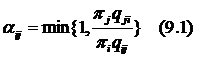
• With probability (9.1), if u <= α_ij, set X_t+1 = j, else set X_t+1 = i.

Such algorithm randomly attempts to move about the sample space, sometimes accepting the transitions and sometimes remaining in the same state. Acceptance ratio indicates how probable the proposed sample is in respect to the current sample. If the next state is more probable than the current, the transition is always accepted. If the next step is less probable, it will be occasionally accepted, but more often rejected. Intuitively, this is why this algorithm works, tending to stay away from the regions with low-density and mostly remaining in the high-density regions.

A key issue in the successful implementation of the algorithm is the number of steps until the chain approaches stationarity, which is called the burn-in period. Typically first 1000 to 5000 elements are thrown out and then a test is used to assess whether stationarity has been reached.

3.4. Gibbs Sampling

Gibbs sampling is a special case of Metropolis-Hastings sampling where the random value is always accepted. The key is the fact that only distributions where all random variables but one are assigned fixed values are considered. The benefit is that such distributions are much easier to simulate compared to complex joint distributions. Instead of generating a single n-dimensional vector in a single pass, n random variables are simulated sequentially from the n conditionals.

A Gibbs stopper is an approach to convergence based on comparing the Gibbs sampler and the target distribution. Weights are plotted as a function of the sampler iteration number. As the sampler approaches stationarity, the distribution of weights is expected to spike.

4. Example

4.1. Initial Data

Table 1 contains the field goal shooting record of LeBron James for the seasons 2003 to 2009. The goal of the simulation was to use OpenBUGS to carry out a MCMC Bayesian simulation and produce a posterior distribution to the probability of the player’s shooting success.

Table 1 – LeBron James Goal Shooting Record

4.2. The Model

The model for the success probabilities of LeBron James is given by (10)

where k = 2, ..., 7, corresponding to seasons from 2004/5 to 2009/10, and π₁ is estimated individually as a success probability for 2003/4 season. R_k are performances for the current seasons. A beta prior is the success probability for the first season and gamma priors are relative successes R_k.

Likelihood for this model is given by (11).

The likelihood is written in OpenBUGS as

for (k in 1:YEARS){ y[k]  ~ dbin( pi[k], N[k] ) }

while the model for success probabilities is expressed as follows:

for (k in 2:YEARS){ pi[k]<-pi[k-1]*R[k] }

The data for the model specifies the values of the successes and total attempts (y_i and N_i) for each season. Initial values for the model must be specified for π₁ and R_k as follows:

list(pi=c(0.5, NA, NA, NA, NA, NA, NA), R=c(NA, 1,1,1,1,1,1))

No initial values were specified for π₂ ... π₇ since they are deterministic and for R₁ since it is constant. Actual initial data used for the model is attached as separate initX.txt files, where X is the number of the chain.

4.3. One Chain Calculation

The initial calculation was run with 1000 samples burn-in and 2000 sample points, for one chain. The posterior summaries were presented in Figure 1

Figure 1 – Posterior summaries for one chain calculation

From these results, the expected success rates for James LeBron was 42.24% for the season of 2003/4, increased by a factor of 1.1 for the season of 2004/5, then stayed close to the level of 2003/4 season for the next 2 seasons (posterior means for R₃ = 1.036 and R₄ = 0.9863) and then was increasing steadily for the next 3 seasons.

Since R_i indicates the relative performance of a current season in comparison to the previous one, it can be reported that the player was steadily increasing his performance over the duration of the seven season, with one especially significant increase of 10.5% early in the career.

Further, posterior distributions of the relative performance vector R were analysed by using the Inference -> Compare function and producing the boxplot, which is presented in Figure 2.

Figure 2 – The boxplot of R

The limits of boxes represent the posterior quartiles and the middle bar – the posterior mean. The endings of the whisker lines are 2.5% and 97.5% posterior percentiles.

Posterior density can be estimated by plotting the success rate density for a season. Figure 3 represents the posterior density for each season (π_i)

Figure 3 – Posterior density for each season

Checking convergence is not a straightforward task. While it is usually easy to say when the convergence definitely was not reached, it is difficult to conclusively say if the chain has converged. Convergence can be checked by using the trace option from Inference -> Samples menu. Figure 4 represents the history plots for π_i.

Figure 4 – History Plots for π_i, one chain

It is clear that π₇ has converged, while the result for other seasons is not so obvious. Multiple chain calculation with a higher number of iterations may be helpful. Another reason to use the higher number of iterations is the reduction of Monte Carlo error in case it is too high – it decreases as the number of iteration grows. In fact, the value of Monte Carlo error can be used to decide when to stop simulation.

4.4. Multiple chain calculation

The main difference between the single and multiple chain calculations is the fact that a separate set of initial values is required for each chain. The following initial values were used for the three chains:

list(pi=c(0.5, NA, NA, NA, NA, NA, NA), R=c(NA, 1,1,1,1,1,1))
list(pi=c(0.9, NA, NA, NA, NA, NA, NA), R=c(NA, 1,1,1,1,1,1))
list(pi=c(0.1, NA, NA, NA, NA, NA, NA), R=c(NA, 1,1,1,1,1,1))

The posterior statistics for this calculation were presented in Figure 5.

Figure 5 – Posterior summaries for multiple chain calculation

The trace plots now contain one line for each chain. The history plots for π_i for this calculation were presented in Figure 6.

Figure 6 – History Plots for π_i, multiple chains

References

Ntzoufras I, Bayesian Modeling Using WinBUGS, 2009, Wiley, England

Reich B, Hodges J, Carlin B, Reich A, A Spatial Analysis of Basketball Shot Chart Data, 2005, NSCU Statistics

Walsh B, Markov Chain Monte Carlo and Gibbs Sampling, 2004, MIT Lecture Notes

Mathematics for Metabolic Modelling - Course Materials 2012, University of Manchester, UK

by Evgeny. Also posted on my website

Building a model for the mouse response to Trypanosoma Congolense using jActiveModules and BiNGO

1. Introduction

African trypanosomes are protozoan parasites that cause severe diseases in human and livestock with fatal consequences unless treated. Trypanosomiasis caused by T. congolense and T. vivax is one of the most significant constraints on cattle production in Africa.

Trypanosomes are extracellular parasites that survive in the bloodstream. In cattle, anaemia is the key feature of the disease and persists after the first wave when parasite numbers have declined to low or undetectable levels. Because of the importance of the anaemia in trypanosomiasis many studies have been carried out to describe its nature and discover its causes (Noyes et al, 2009).

A mouse model may be helpful in developing understanding of the mechanisms underlying the resistance to trypanosoma. Certain strains of mice are tolerant to the disease while others are highly susceptible. Microarray experiments have been carried out on C57BL/6, BALB/c and A/J strains of mice. A large amount of data has been recorded at different time points after the infection.

2. Background

The microarray experiment results were provided for this project in the form of an interaction network (hereafter “mouse liver” network) including only those genes for which there is evidence of expression in liver. The data was provided in the form of xgmml file. The data showing the changes in gene expression between day 0 and day 7 post-infection was measured on samples from liver tissue and was provided in the form of the pvals file.

3. Aims

The aim of the project was to examine the data provided at the pathway level. A possible model was developed for the mouse response at peak parasitaemia (day 7 after infection).

4. Materials and methods

The following software was used in the project:

• Cytoscape version 2.8.2
• Network Analysis plugin
• Advanced Network Merge plugin
• jActiveModules plugin

The following data was provided:

• Mouseliver.xgmml : the interaction network file
• Abc07.pvals : the gene expression file

The data was analysed using the software listed above following the protocol by Cline et al (2007).

4.1. Network parameters

The mouse liver network was loaded into Cytoscape. The network contained 3,531 nodes and 17,195 edges (Figure 1). The network consisted of one large connected component of 2,674 nodes and 15,639 edges and 253 smaller components not connected to the large component. The smaller components range in size from 2 to 36 nodes.

Figure 1 - Mouse liver network.

4.2. Node Degree Distribution

As expected from literature, node degree distribution in a cellular network is not random, but follows a power law (Barabasi & Oltvai, 2004). The power law was fitted as follows: y = 6578x^-1.918. The power law explains 91.6% of the distribution, which is a very good fit (Figures 2, 3).

Figure 2 - Node degree distribution and power law

Figure 3 - Node degree distribution

The value of betweenness centrality is normalized and therefore lies between 0 and 1.

Figure 4 - Betweenness centrality in mouse liver network

4.3. Identifying Active Modules

Gene expression data was imported into Cytoscape from the abc07.pvals file provided. The significance values a07sig, b07sig and c07sig were used to identify active modules within the mouse liver network using the jActiveModules plugin. The plugin identified five active modules. Two first modules, containing 185 and 234 nodes, were selected for further analysis. The Advanced Network Merge plugin was used to identify the intersection between the modules. The resulting merged network contained 143 nodes, which is a high degree of intersection.

The following steps were performed for each module and for the intersection network:

• expression data was coloured by fold change in A/J mice
• ten proteins with highest log fold values were identified
• the results were presented in Tables in results section, including protein name, log fold value and whether the protein is present in module 1, module 2 and the intersection between modules

The steps were repeated for BALB/c and C57BL/6 mice strains.

Figure 5 - Active module identified in mouse liver network.

4.4. Checking against Gene Ontology

Gene ontology project provides a controlled vocabulary of terms for describing gene product characteristics and gene product annotation data. Gene Ontology for the mouse liver network was checked using the BiNGO plugin v. 2.44. The following files were downloaded from the Gene Ontology website: the full ontology file v.1.2 (gene_ontology_ext.obo) from the downloads/ontologies section and Mus musculus annotation file (gene_association) from downloads/annotations section.

• BiNGO plugin was started
• With the whole mouse liver network being active, the first of the active modules found in 4.3 was selected. This highlighted the module nodes in the mouse liver network
• The following settings were changed from default in BiNGO settings screen:
• Select reference set: “Use Network as Reference set”
• Select ontology file: gene_ontology_ext.obo
• Select organism/annotation: gene_association
• Significance level: 0.01
• BiNGO analysis was performed
• BiNGO output in the form of the data panel and the graph was analysed and the results were investigated in the attempt to identify the gene categories that were over-represented.

The steps above were repeated for the second active module.

Two categories were identified as over-represented for further analysis. The genes annotated with these categories were selected from the original mouse liver network into new networks. Each of these networks was then analysed to find the intersection between the over-represented category and the active modules identified in 4.3.

5. Results

The output from the BiNGO plugin was analysed and the genes with the highest log fold values on day 7 were presented in the tables below, broken down for mouse strains and indicating if the gene is present in module 1, module 2 and the intersection network.

Gene	a07exp	Module 1	Module 2	Intersection
Ubd	5.9678954	1	1	X
Gbp2	5.7735786	2	2	X
Ccl8	5.7155864		3
Gbp1	5.445365	3	4	X
Lgals3	5.4172534	4	5	X
Serpina3g	5.362374	5	6	X
Ccl6	5.1455947	6	7	X
Marco	5.030731	7	8	X
Fpr2	4.822051	8
Mmp13	4.6918998		9
Cxcl9	4.5458629	9	10	X
Gzmb	4.5131922	10	11	X

Figure 6 - Genes with highest log fold values in A/J strain, day 7

Gene	b07exp	Module 1	Module 2	Intersection
Serpina3g	6.76103175	1	1	X
Gbp2	5.82087485	2	2	X
Gbp1	5.7275038	3	3	X
Fpr2	4.94588325	4
Lgals3	4.90982775	5	4	X
Cd74	4.78939395	6	5	X
Ly6a	4.7619165	7	6	X
Ccl8	4.62952825		7
H2-Aa	4.624156175	8	8	X
Fcgr4	4.5432714	9	9	X
H2-Eb1	4.4276222	10	10	X

Figure 7 - Genes with highest log fold values in BALB/c strain, day 7

Gene	c07exp	Module 1	Module 2	Intersection
Ubd	6.4093402	1	1	X
Gbp2	6.2236	2	2	X
Serpina3g	5.1775226	3	3	X
Cxcl9	5.0992863	4	4	X
Cxcl10	4.7095646	5	5	X
Lgals3	4.6491436	6	6	X
Gbp1	4.2545664	7	7	X
Igj	4.2137042		8
Fpr2	4.1394768	8
Gzmb	3.7592078	9	9	X
Vim	3.7421474	10	10	X

Figure 8 - Genes with highest log fold values in C57BL/6 strain, day 7

Graphical output from BiNGO was analysed visually. The yellow and orange nodes represent gene ontology categories that are overrepresented at the significance level. Uncoloured nodes are not overrepresented themselves, but they are parents of overrepresented nodes further down. Some nodes could be immediately identified as most relevant – there were most intensely coloured and were located away from the centre of the network. Nodes with GO-ID 6954 (inflammatory response) and 9611 (response to wounding) were selected as relevant.

Figure 9 - BiNGO output for active module 1 and nodes with GO-ID 6954, 9611

Figure 10- BiNGO output for active module 2 and nodes with GO-ID 6954, 9611

Next, genes annotated as “inflammatory response” and genes annotated as “response to wounding” were selected as new networks.

Figure 11 - Genes annotated as 'inflammatory response' (GO-ID 6954)

Figure 12 - Genes annotated as 'response to wounding' (GO-ID 9611)

Finally, the intersection of the annotated genes and the active modules was analysed.

Figure 13 - Genes annotated as 'inflammatory response' (GO-ID 6954) in active module 1

Figure 14- Genes annotated as 'response to wounding' (GO-ID 9611) in active module 1

Figure 15 - Genes annotated as 'inflammatory response' (GO-ID 6954) in active module 2

Figure 16 - Genes annotated as 'response to wounding' (GO-ID 9611) in active module 2

6. Discussion

Scientists have studied a mouse model of tolerance to trypanosomiasis. C57BL/6 mice survive for a relatively long period after infection with T. congolense (110 days), strains such as A/J (16 days) or BALB/c (49 days) are relatively susceptible (Goodhead et al., 2010).

Hanotter et al (2003) aimed to identify Quantitative Trait Loci (QTL) that control resistance to trypanosomiasis in cattle. They made an experimental cross between trypanotolerant African N'Dama (Bos taurus) and tryptanosusceptible Kenya Boran (Bos indicus). They genotyped 177 animals and their parents and grandparents at 477 molecular marker loci covering all autosomes, covering 82% of the genome. The analysis supported a multilocus model for the inheritance of trypanotolerance and ten QTL were identified as contributing to disease tolerance. The location and structure of the QTL regions was determined by using public Single Nucleotide Polymorphisms (SNP) and identifying where the SNPs correlated with survival time in species.

Kemp et al (1997) genotyped crosses between resistant and susceptible mouse breeds and identified the loci on the chromosomes that had a significant effect on survival time. They identified three major QTL that determined the outcome of trypanosome infection in mice and called them Tir1, Tir2 and Tir3.

Fisher et al (2007) suggested the workflows that combine Microarray and QTL data to search for candidate genes responsible for phenotypic variation. The workflows were applied to the case of resistance to trypanosomiasis in the mouse. An initial list of 344 genes identified in the Tir1 QTL region has been narrowed down to 32 candidate genes. Further, MapK signalling pathway was identified as containing a high proportion of genes that show differential expression. Daxx showed the strongest signal of differential expression and was chosen as the primary candidate.

Goodhead et al (2010) applied a series of analyses to existing datasets and combined them with novel sequencing and other genetic data to create short lists of genes that share polymorphisms across susceptible mouse breeds. They reduced the initial long list of genes within the QTL regions to a short list of candidate genes with defined genetic differences that correlate with phenotype. Pram1 regulates oxidative stress in neutrophils and Rgl2 is involved in Ras signalling which can regulate inflammation. Pram1 has the best understood functionality and Rgl2 is also a plausible candidate. Probably damaging polymorphisms were identified in Srp72 and Thsd7b but little is known of their functions making interpretation hard. Ptprc and Soat1 had probably damaging polymorphisms. Cd244 is differentially expressed and has a haplotype that correlates with phenotype in the four strains tested.

Goodhead et al (2010) identified Pram1 as the most plausible candidate gene in Tir1. They also identified Cd244 as a strong candidate gene in the Tir3 QTL. Pram1 has several GO annotations, which are “lipid binding”, “regulation of neutrophil degranulation” and “integrin-mediated signalling pathway”. Cd244 is annotated as “natural killer cell receptor 2B4”.

Pram1 is an intracellular adaptor that is critical for select integrin functions in neutrophils, which are critical for host defence against pathogens (Clemens et al, 2004). From the comparison of the log fold changes for Pram1 in three strains it can be noticed that the value for C57BL/6 is almost three times greater than for A/J and 48 times greater than for BALB/c. However, the absolute value of log fold for Pram1 is not outstanding compared to other genes. This suggests that it is not the absolute value of the log fold that is important, but the difference in the log folds for the same gene across three mouse strains. Pram1 was not picked up as part of the active module by the jActiveModules plugin. Consequently, Pram1 could not appear in the output of the BiNGO plugin, suggesting that the technique used may not be optimal for identifying the genes responsible for disease resistance.

Cd244 is expressed on all Natural Killer cells in mice. It mainly acts as an inhibitory receptor and this function plays a role in maintaining tolerance of Natural Killer cells to self cells (Vaidyaa & Mathew, 2006). Cd244 was identified by the jActiveModules plugin as part of active module 2. It should be noted that for this gene the log fold values is lower in the tolerant C57BL/6 strain compared to two other strains. However, the GO annotation for Cd244 did not appear in the output of the BiNGO plugin. The likely explanation is that it was not picked up by the plugin due to low significance values.

Gene	a07exp	a07sig	b07exp	b07sig	c07exp	c07sig
Pram1	0.129875	0.644749889	0.00729335	0.978568283	0.3465516	0.232430853
Cd244	2.020997	9.93E-7	1.2643455	1.81269E-4	0.6374838	0.382130858

Figure 17 - Significance and expression values for Pram1 and Cd244

Fisher et al (2007) identified an amino acid deletion in the Daxx gene in susceptible mouse strains and proposed Daxx as a candidate gene in the Tir1 Q TL region. Daxx is annotated as “Death domain-associated protein 6”. Daxx accumulates in both the nucleus and the cytoplasm and has been reported to interact with various proteins involved in cell death regulation. Its precise role in cell death is only partially understood despite a number of studies on the subject (Salomoni & Khelifi, 2006). Daxx was also not identified by jActiveModules as part of the active module in the mouse liver network.

7. Conclusion

This document describes an attempt to build a model for the mouse response to the infection by Trypanosoma congolense. A large amount of data from microarray experiments is loaded as an interaction network into Cytoscape and then analysed using the jActiveModules and BiNGO plugins. The use of the protocol described in this document allows suggesting several candidate genes but the results are not supported by literature and previous research.

The BiNGO plugin allows to determine which Gene Ontology terms are overrepresented in the set of genes (Maere, Heymans and Kuiper, 2005). It provides the output both as a data table and a visual graph. The visual graph, however, is subject to interpretation and it is hard to determine which nodes in the graph are of the most interest. Maere, Heymans and Kuiper (2005) note that interpretation can be difficult if a whole branch of the GO hierarchy is highlighted as being significantly overrepresented, which is very likely due to the interdependency of functional categories. It should be added that in more complex networks, even when the least significant nodes are not considered, multiple branches may be highlighted as being overrepresented, further complicating the visual analysis.

Additionally, identifying the nodes of interest only gives a reference to a GO category, which may include a large number of genes. If the goal is to reduce the amount of candidate genes to a number under ten, identifying the overrepresented category would only be one of the first steps.

While BiNGO is a tool that is flexible and easy to use, its application to the identification of the genes that play a key role in the resistance to a disease is only part of a high-level analysis. Other techniques and workflows will be needed that can use the BiNGO output and use it to further refine the list of candidate genes.

8. References

A-L Barabasi, Z. Oltvai, Network biology: Understanding the cell's functional organization, Nature Reviews Genetics, 5:101 (2004)

R. Clemens, S. Newbrough, E. Chung, S. Gheith, A. Singer et al, PRAM-1 Is Required for Optimal Integrin-Dependent Neutrophil Function, Molecular and cellular biology, 24:10923 (2004)

M. Cline, M. Smoot, E. Cerami, A. Kuchinsky, N. Landys et al., Integration of biological networks and gene expression data using Cytoscape, Nature protocols 2:2366 (2007)

P. Fisher, C. Hedeler, K. Wolstencroft, H. Hulme, H. Noyes et al, A systematic strategy for large-scale analysis of genotype–phenotype correlations: identification of candidate genes involved in African trypanosomiasis, Nucleic Acids Research, 35:5625 (2007)

Gene Ontology website, accessed on 07/01/2012

I.Goodhead, A. Archibald, P. Amwayi, A. Brass, J. Gibson et al, A Comprehensive Genetic Analysis of Candidate Genes Regulating Response to Trypanosoma congolense Infection in Mice, PLoS Neglected Tropical Diseases 4(11): e880 (2010)

O. Hanotte, Y. Ronin, M. Agaba, P. Nilsson, A. Gelhaus et al, Mapping of quantitative trait loci controlling trypanotolerance in a cross of tolerant West African N'Dama and susceptible East African Boran cattle, Proceedings of the National Academy of Sciences of the United States of America, 100:7443 (2003)

S. Kemp, F. Iraqi, A. Darvasi, M. Soller and A. Teale, Localization of genes controlling resistance to trypanosomiasis in mice, Nature genetics, 16:194 (1997)

S. Maere, K. Heymans and M. Kuiper, BiNGO: a Cytoscape plugin to assess overrepresentation of Gene Ontology categories in Biological Networks, Bioinformatics Applications, 21:3448 (2005)

H. Noyes, M. Alimohammadian, M. Agaba, A. Brass, H. Fuchs et al., Mechanisms Controlling Anaemia in Trypanosoma congolense Infected Mice, PLoS ONE 4(4): e5170 (2009).

P. Salomoni, A. Khelifi, Daxx: death or survival protein?, Trends in cell biology, 16:97 (2006)

S. Vaidyaa, P. Mathew, Of mice and men: Different functions of the murine and human 2B4 (CD244) receptor on NK cells, Immunology letters 2:180 (2006)

Feedback from the Tutor

The aims are rather too broad; you could focus more specifically on the strain differences. The overall strategy is clear and sensible, but each figure needs a full legend giving the colour scheme used. You have provided a full discussion, but it is organised as 'literature and then my results'. In a report of this type you need to discuss your own results, and then consider whether there is supporting evidence from the literature. List the references with surname first.

by Evgeny. Also posted on my website