Sunday, December 25, 2011

Adding Expression Data to the Network

Introduction

The network that I have been using is a generalised view of the interactions that may take place. By adding gene expression data to the network, I will be able to determine which interactions are 'active' under the known experimental conditions. The data provided for analysis was from an experiment to examine the changes in gene expression in the lungs of rats exposed to mustard gas (GSE1888).

The goal was to find, identify and compare the active modules and how they overlap with the network of proteins affected by mustard gas.

1. Functional Modules

When the protein interactions are represented as graphs, they can be used to investigate the functions of proteins through their interactions with neighbouring proteins. Clusters of highly interconnected proteins could not have occurred by chance and are likely to contain proteins with a common biological function (Dunn et al, 2005). Such clusters are called functional modules and their identification is a complex task.

Bader and Hogue (2003) suggested the three-stage algorithm for finding molecular complexes. The algorithm assigns weights to nodes based on “cliquishness” of a node, which is proportional to the number of nodes in the neighbourhood and inversely proportional to the vertex size of the neighbourhood.

Dunn et al. (2005) note that in certain cases, such as a prey node attached to the bait by a single edge, a poorly connected node provides useful information. Methods that use edge-betweenness, unlike many other clustering methods, will not remove such nodes and are useful when the information associated with these low degree nodes is required.

2. Finding Active Modules

The file provided for the exercise contained significance values of the difference in gene expression in rats that were exposed to 6mg/kg mustard gas for 1, 3 and 6 hours. The jActiveModules plugin was used to find active modules. The plugin identified five functional modules ranging from 69 to 95 nodes in size.

3. Examining Active Modules

Network from module 1.

1 hour: all significance values are equal to 0.999783355
3 hours: significance values in range of 4.5*10-5 to 0.489861449

Graphical view, with nodes having higher significance values coloured with darker red.

In this network, only five proteins have significance values over 0.01.

6 hours: significance values in range of 6.13*10-8 to 0.916047284

This time, over 30 proteins have significance values over 0.01.

Network from module 2.

1 hour: all significance values are equal to 0.999783355

3 hours: significance values in range of 4.5*10-5 to 0.489861449

6 hours: significance values in range of 6.13*10-8 to 0.916047284

4. Comparing the Modules Identified

After networks were created from first three of the five active modules identified, the Cytoscape plugin Advanced Network Merge was used to merge these three modules.

The merged network which is coloured according to the differential expression at 6 hours was represented on the image below:

It is not immediately obvious from the picture how strongly the three networks which were merged into one overlap. One observation is that the merged network has 118 nodes, while the three child networks would have 95 + 44 + 72 = 211 nodes if there was no overlap. This is an indication that a significant number of nodes are present in two or three child networks.

Another approach may be to compare the proteins with high p-values. To fill the table below, the nodes in each of the child active modules were sorted by p-value at 6 hours. Then ten proteins with highest p-values were inserted into the table. One protein (Icam1) was present in all three “top tens”. Module 1 and 2 share one other protein (Krt19), and modules 1 and 3 share one other protein (Lpl), while modules 2 and 3 share five other proteins (Cd36, Hamp, Sacm11, Tim3, Dusp1). From this basic analysis it can be roughly estimated that all three modules are overlapped to some extent, and modules 2 and 3 are more significantly overlapped compared to module 1 and 2 or 1 and 3. Further more detailed analysis is required to make more exact conclusions.


Active Module 1Active Module 2Active Module 3
LplLpl
Sele
Icam1Icam1Icam1
Il18
Krt19Krt19
Nr1h3
Pla2g1b
Col5a2
Nt5e
Pawr
Axin1
Cd36Cd36
HampHamp
Sacm1lSacm1l
Timp3Timp3
Mark3
Dusp1Dusp1
Phlda1
Pcm1
Raf1
Gsk3b

References:

R. Dunn, F. Dudbridge, C. Sanderson, The Use of Edge-Betweenness Clustering to Investigate Biological Function in Protein Interaction Networks, BMC Bioinformatics, 6:39 (2005)

G. Bader, C. Hogue, An automated method for finding molecular complexes in large protein interaction networks, BMC Bioinformatics, 4:2 (2003)

Feedback

You have identified and shaded active modules. However, it is more interesting at this stage to shade by fold change, rather than by significance value. By using the fold change values (1hexp, 3hexp, 6hexp) you can see which parts of your network are up/down-regulated over the course of the experiment. In the practical instructions I suggested that you use the intersection option when merging your networks. This does show you the extent of the overlap.

My Comment

It was quite stupid of me to use 'union' instead of 'intersect' when merging networks and then record that there are no obvious observations.

by . Also posted on my website
Thursday, December 15, 2011

Network Topology

Degree distribution and power law.

For a long time the graph theory modelled complex networks either as being regular objects, or as being completely random. An important finding was that the number of nodes with a given degree does not follow the Poisson distribution, but follows a power law (Barabasi & Oltvai, 2004)

That means that the probability to find a hub with a number of neighbours a magnitude higher is a magnitude lower, but still not negligible (Bode et al, 2007).

In simple terms, a node with a degree of 10 will be found 10 times less often, than the node with a degree of 1, and the node with a degree of 100 - 100 times less often.

Such networks are called scale-free, which means that it is not possible to find a typical node in the network - one that could be used to characterize the rest of the nodes. The evidence that cellular networks are scale-free came from the analysis of metabolism networks of various organisms. As a typical feature of the scale-free network, most of the proteins only participate in a few interactions, but there is a small number of proteins which participate in dozens interactions. Alternatively it can be described as a small number of hubs (highly connected nodes) which hold the whole network together. (Barabasi & Oltvai, 2004)

From the evolutionary point of view, there are two factors that explain scale-free nature of cellular networks. One is the fact that most network are a result of a very slow growth over an extended time period, and the other is that new nodes are more likely to connect to nodes which already have many links. (Barabasi & Oltvai, 2004)

Not everyone agrees to the fact that the node degree distribution follows a power law. Tanaka et al (2005) studied the two publicly available networks, the FYI (filtered yeast interactome) and human protein interaction (HPI) maps and investigated whether their node degree sequences follow a power law. Their conclusion was that usage of frequency-degree plots leads to errors which can easily be avoided by using rank-degree plots and the node degree sequences of these networks are clearly not power laws, but much closer to exponential.

Betweenness Centrality

Betweenness is a quantitative measure for describing the centrality of nodes in a network, provided as the frequency with which a node is located on the shortest path between all other nodes. Nodes with high betweenness control the flow of information across a network. There is a positive correlation between the centrality of the proteins and their essentiality in many species, and there is also a positive correlation between centrality and node degree. (Yamada & Bork, 2009)

Betweenness centrality lies at the core of both transport and structural vulnerability properties of complex networks; however, it is computationally costly, and its measurement for networks with millions of nodes is nearly impossible. (Ercsey-Ravasz & Toroczkai, 2010).

One of the practical applications of betweenness centrality is the drug design. Hormozdiari et al (2010) suggest that if the essential pathways in a pathogenic organism are known, it should be possible to compute the minimum number of proteins that need to be targeted as many essential pathways as possible. The proteins with the highest betweenness will be the most obvious choices but, of course, the algorithm is not that simple and includes a schema whether the proteins are also weighted based on the presence of an ortholog of a protein in the host. We wouldn't want a drug to target vital proteins in our own body.

Calculating and using network statistic.

Node degree distribution

It is evident that there is a large number of nodes with a low node degree, but there is only a handful of nodes with a degree over 100. The degree distribution does not appear to be random and it is known from literature that it usually follows a power law.


Figure 1 – node degree distribution in a large network.

Fitting a power law.

The power law was fitted as follows: y=3391.6 * x-1.698. The power law explains 92.5% of the distribution, which is a very good fit. This is also evident from the fact that the residues appear to be distributed randomly to the both sides of the fitted line and close to the line.


Figure 2 – power law fitted functionFigure 3 – power law fitted graph.

Betweenness centrality

The value of betweenness centrality is normalized and therefore lies between 0 and 1.

Figure 4 – betweenness centrality in a large network.

Removing the largest component.

The largest connected component in the network being studied has 2623 nodes, which is the majority of the nodes of the whole network and the largest of the other components is only 12 nodes.

Figure 5 – largest connected components of a large network.

Below is the second largest of components, with the node marked in yellow having a high betweenness centrality of 0.7:

Figure 6 – second largest connected component of large network

This node connects two “clusters” of 5 and 4 nodes, and two other nodes. Since the definition of betweenness is “number of shortest paths from all nodes to all others that pass through that node”, it has a relatively high betweenness.

Several example nodes from the largest connected components:

A node with high betweenness centrality (0.082), high degree (150) : Cam1. The node has a high degree, so it is connected to many other nodes in the network. Therefore a significant number of shortest paths passes through the node. It can also be seen that a significant number of nodes other than Cam1 are directly connected to each other, reducing the betweenness of Cam1.

Figure 7 – Cam1 and neighbouring nodes.

A node with relatively high betweenness centrality (0.01), low degree (10) : Csnk2b. This one is not obvious to me, I would expect the betweenness of this node to be higher since it appears to be central to its five neighbours. Probably as part of the whole connected component it belongs to the peripheral area of the network.

Figure 8 – Csnk2b and neighbouring nodes.

A node with low betweenness centrality (0), relatively high degree (28) : Ndufb8. Nodes other than Ndufb8 are highly connected, so only a small number of shortest paths between nodes pass through Ndufb8.

Figure 9 – Ndufb8 and neighbouring nodes.

A node with low betweenness centrality (0), low degree (4) : Fbxo11. There is only one node here other than Fbxo11, so there are no routes between nodes other than Fbxo11 at all.

Figure 10 – Fbxo11 and neighbouring nodes.

References:

A-L Barabasi, Z. Oltvai, Network biology: Understanding the cell's functional organization, Nature Reviews Genetics, 5:101 (2004)

T. Yamada, P. Bork, Evolution of biomolecular networks - lessons from metabolic and protein interactions, Nature Reviews Molecular Cell Biology, 10:791 (2009)

R. Tanakaa, T. Yi, J. Doyle, Some protein interaction data do not exhibit power law statistics. FEBS Letters, 579:514 (2005)

C. Bode, I. Kovacs, M. Szalay, R. Palotai, T. Korcsmaros et al., Network analysis of protein dynamics, FEBS Letters, 581:2776 (2007)

M. Ercsey-Ravasz, Z. Toroczkai, Centrality scaling in large networks, Physical review letters, 105:38701(2010)

F. Hormozdiari, R. Salari, V. Bafna, S. Sahinalp, Protein-protein interaction network evaluation for identifying potential drug targets, Journal of Computational Biology, 17:669 (2010)

by . Also posted on my website
Wednesday, December 7, 2011

Starting With Cytoscape

Cytoscape is a popular open source platform for visualising molecular interaction networks.

Cytoscape website

Cytoscape has a built-in plugin manager (Plugins -> Manage Plugins) which lets the user install a large number of plugins.

One of the most important applications of Cytoscape is the analysis of interaction networks. The networks are described by eXtensible Graph Markup and Modeling Language - XGMML.

XGMML

I found a sample file here

pte.xgmml

To import the file into Cytoscape, select File -> Import -> Network(multiple file types)

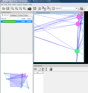
This is how a network typically may look.

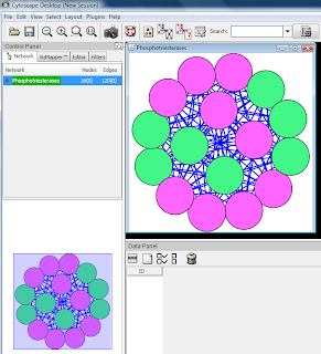
To view all nodes and edges, apply a layout, for example Layouts -> Cytoscape Layouts -> Spring Embedded

In the Node Attribute Browser below, click "Select All Attributes". To select all nodes in the Cytoscape model, use Ctrl-A.

If the network is large, it is possible to use a selection criteria to select nodes of interes and to create a new network from the selected nodes only. For example, it is possible to sort the nodes by an attribute in the node attribute browser (or edge attribute browser), select a number of nodes and then select File -> New -> Network -> From Selected Nodes, All Edges. Cytoscape will create a child subnetwork which will only include selected nodes and/or edges.


by . Also posted on my website