Markov Chains Monte Carlo Bayesian Inference

1. Bayesian Inference

Bayesian rule is a mathematical rule that explains how the estimate of the probability changes as new evidence is collected. It relates the odds of event A₁ to event A₂ before and after conditioning on event B (1).

As an example, assume that there is a bag containing black and white balls, but the percentage of colours is unknown. As more and more balls are drawn from the bag, the probability of the next ball being white (or black) can be calculated with higher precision. In this case, A₁ is the probability of white ball being drawn, A₂ of the black ball, and B is the set of the balls already drawn, such as “of 10 balls 4 were black and 6 were white”.

Frequentist approach to Bayes’ rule is to consider probabilities of A₁ and A₂ as known and fixed, while in Bayesian they are considered random variables. Bayesian approach also considers prior probability, or just the prior, which expresses uncertainty before the data is taken into account. It makes possible to introduce subjective knowledge of the problem into the model in the form of prior information. Among the drawbacks of the approach is the need to evaluate multi-dimensional integrals numerically, which gets worse as the number of parameters in the system increases. Introduction of conjugate prior is an attempt to solve these drawbacks. Conjugate prior is such prior distribution that the prior and posterior are in the same family of distributions. Markov Chains are useful because under certain conditions, a memoryless process can be generated which has the same limiting distribution as the random variable that the calculation is trying to simulate.

2. Markov Chains

A Markov chain is a process which can be in a number of states. The process starts in one of the states and moves successively from one to another. Each move is called a step. At each step a process has a probability to move to another state, and the probability does not depend on any of the previous states of the process. That is why such process is called “memoryless”.

Example: In a weather model, a day can be either nice, rainy or snowy. If the day is nice, the next day will be either rainy or snowy with 50% probability. If the day is rainy or snowy, it will stay the same with 50% probability, or will change to one of the other two possibilities with 25% probability. This is a Markov chain because the process determines its next state base on the current state only, without any prior information. The probabilities can be presented in the transition matrix (2).

The first row presents the probabilities of the next day’s weather if today is rainy (R): ½ that it will remain rainy, ¼ that it will be nice and ¼ that it will be snowy. The sum of probabilities across the row must be equal to 1.

3. Monte Carlo Methods

Markov Chains Monte Carlo (MCMC) methods are computational algorithms which randomly sample from the process. The aim of the methods is to estimate something that is too difficult or time consuming to find deterministically. Using the example above, assume that the probabilities in the matrix are not known. A MCMC could simulate a thousand rainy days and count the number of snowy, rainy and nice days that follow. The same could be repeated for snowy and nice days.

The original Monte Carlo approach was developed to use random number generation to compute integrals. If a complex integral can be decomposed into a function f(x) and a probability density function p(x), then the integral can be expressed as an expectation of f(x) over the density p(x) (3)

Now, if we draw a large number of x₁, ..., x_n of random variables from the density p(x), then we end up with (4), which is referred to as Monte Carlo integration.

3.1. Markov Chain Convergence

It can be shown that if matrix P is the transition matrix for a Markov chain and p_ij element is the probability of transitioning from state i to state j, then the element p_ij⁽ⁿ⁾ of the matrix Pⁿ gives the probability that the Markov chain starting in state s_i will be in state s_j after n steps. Using the transitional matrix (2), on the sixth step of multiplying the matrix by itself the following state will be reached (5). Such Markov chain is called regular (not all Markov chains are regular). The long-range predictions for this chain are independent of the starting state.

Continuing the example, assume that the initial probabilities for the weather conditions on the starting day of the chain are equal. This will be called a probability vector, which in the example will be as shown in (6).

It can be shown that the probability of the chain being in the state s_i after n steps is the ith entry in the vector (7).

If, as in the example, the chain is regular, it will converge to a stationary distribution, when the probability of the chain being in state i is independent of the initial distribution. In the weather example, the stationary distribution is shown in (8).

3.2. Ergodicity and Reversibility

If the process that starts from state i will ever re-enter state i, such state is called recurrent. Additionally, such state is called nonnull if it re-enters state i in n steps, where n is finite. A process is called aperiodic if the greatest common divisor of return steps to any state is 1. For example, if the chain re-enters a state after 2, 4, 6 steps and so on, such chain is not aperiodic. A process is called irreducible if any state can be reached from any other state in a finite number of moves. A chain that is recurrent nonnull, aperiodic and irreducible is called ergodic, and the ergodic theorem states that a unique limiting distribution exists for the chain and such distribution is independent of initial distribution.

A Markov chain is reversible if (9) is satisfied for all i, j, where u is the stationary distribution and p_ij are elements of the transition matrix.

Ergodicity and reversibility are the two principles behind the Metropolis-Hastings algorithms.

3.3. Metropolis-Hastings algorithms

One of the problems of applying Monte Carlo integration is in obtaining samples from some complex probability distribution. Mathematical physicists attempted to integrate complex functions by random sampling. Metropolis showed how to construct the desired transition matrix and later Hastings generalized the algorithm. The essential idea of the algorithm is to construct a reversible Markov chain for given distribution π such, that its stationary distribution is π. It starts with generating the candidate j from a proposal transition matrix Q. This matrix Q transitions from current state i to proposal j. Proposal j is then accepted with some probability α_ij. If the rejection takes place, then the next state retains the current value. The summary of the algorithm is as follows:

• Start with arbitrary X₀. Then, at each iteration t = 1, ..., N:
• Sample j~q_ij. Q={q_ij} is the transition matrix.
• Generate u – a uniformly distributed random number between 0 and 1.
• With probability (9.1), if u <= α_ij, set X_t+1 = j, else set X_t+1 = i.

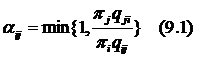
Such algorithm randomly attempts to move about the sample space, sometimes accepting the transitions and sometimes remaining in the same state. Acceptance ratio indicates how probable the proposed sample is in respect to the current sample. If the next state is more probable than the current, the transition is always accepted. If the next step is less probable, it will be occasionally accepted, but more often rejected. Intuitively, this is why this algorithm works, tending to stay away from the regions with low-density and mostly remaining in the high-density regions.

A key issue in the successful implementation of the algorithm is the number of steps until the chain approaches stationarity, which is called the burn-in period. Typically first 1000 to 5000 elements are thrown out and then a test is used to assess whether stationarity has been reached.

3.4. Gibbs Sampling

Gibbs sampling is a special case of Metropolis-Hastings sampling where the random value is always accepted. The key is the fact that only distributions where all random variables but one are assigned fixed values are considered. The benefit is that such distributions are much easier to simulate compared to complex joint distributions. Instead of generating a single n-dimensional vector in a single pass, n random variables are simulated sequentially from the n conditionals.

A Gibbs stopper is an approach to convergence based on comparing the Gibbs sampler and the target distribution. Weights are plotted as a function of the sampler iteration number. As the sampler approaches stationarity, the distribution of weights is expected to spike.

4. Example

4.1. Initial Data

Table 1 contains the field goal shooting record of LeBron James for the seasons 2003 to 2009. The goal of the simulation was to use OpenBUGS to carry out a MCMC Bayesian simulation and produce a posterior distribution to the probability of the player’s shooting success.

Table 1 – LeBron James Goal Shooting Record

4.2. The Model

The model for the success probabilities of LeBron James is given by (10)

where k = 2, ..., 7, corresponding to seasons from 2004/5 to 2009/10, and π₁ is estimated individually as a success probability for 2003/4 season. R_k are performances for the current seasons. A beta prior is the success probability for the first season and gamma priors are relative successes R_k.

Likelihood for this model is given by (11).

The likelihood is written in OpenBUGS as

for (k in 1:YEARS){ y[k]  ~ dbin( pi[k], N[k] ) }

while the model for success probabilities is expressed as follows:

for (k in 2:YEARS){ pi[k]<-pi[k-1]*R[k] }

The data for the model specifies the values of the successes and total attempts (y_i and N_i) for each season. Initial values for the model must be specified for π₁ and R_k as follows:

list(pi=c(0.5, NA, NA, NA, NA, NA, NA), R=c(NA, 1,1,1,1,1,1))

No initial values were specified for π₂ ... π₇ since they are deterministic and for R₁ since it is constant. Actual initial data used for the model is attached as separate initX.txt files, where X is the number of the chain.

4.3. One Chain Calculation

The initial calculation was run with 1000 samples burn-in and 2000 sample points, for one chain. The posterior summaries were presented in Figure 1

Figure 1 – Posterior summaries for one chain calculation

From these results, the expected success rates for James LeBron was 42.24% for the season of 2003/4, increased by a factor of 1.1 for the season of 2004/5, then stayed close to the level of 2003/4 season for the next 2 seasons (posterior means for R₃ = 1.036 and R₄ = 0.9863) and then was increasing steadily for the next 3 seasons.

Since R_i indicates the relative performance of a current season in comparison to the previous one, it can be reported that the player was steadily increasing his performance over the duration of the seven season, with one especially significant increase of 10.5% early in the career.

Further, posterior distributions of the relative performance vector R were analysed by using the Inference -> Compare function and producing the boxplot, which is presented in Figure 2.

Figure 2 – The boxplot of R

The limits of boxes represent the posterior quartiles and the middle bar – the posterior mean. The endings of the whisker lines are 2.5% and 97.5% posterior percentiles.

Posterior density can be estimated by plotting the success rate density for a season. Figure 3 represents the posterior density for each season (π_i)

Figure 3 – Posterior density for each season

Checking convergence is not a straightforward task. While it is usually easy to say when the convergence definitely was not reached, it is difficult to conclusively say if the chain has converged. Convergence can be checked by using the trace option from Inference -> Samples menu. Figure 4 represents the history plots for π_i.

Figure 4 – History Plots for π_i, one chain

It is clear that π₇ has converged, while the result for other seasons is not so obvious. Multiple chain calculation with a higher number of iterations may be helpful. Another reason to use the higher number of iterations is the reduction of Monte Carlo error in case it is too high – it decreases as the number of iteration grows. In fact, the value of Monte Carlo error can be used to decide when to stop simulation.

4.4. Multiple chain calculation

The main difference between the single and multiple chain calculations is the fact that a separate set of initial values is required for each chain. The following initial values were used for the three chains:

list(pi=c(0.5, NA, NA, NA, NA, NA, NA), R=c(NA, 1,1,1,1,1,1))
list(pi=c(0.9, NA, NA, NA, NA, NA, NA), R=c(NA, 1,1,1,1,1,1))
list(pi=c(0.1, NA, NA, NA, NA, NA, NA), R=c(NA, 1,1,1,1,1,1))

The posterior statistics for this calculation were presented in Figure 5.

Figure 5 – Posterior summaries for multiple chain calculation

The trace plots now contain one line for each chain. The history plots for π_i for this calculation were presented in Figure 6.

Figure 6 – History Plots for π_i, multiple chains

References

Ntzoufras I, Bayesian Modeling Using WinBUGS, 2009, Wiley, England

Reich B, Hodges J, Carlin B, Reich A, A Spatial Analysis of Basketball Shot Chart Data, 2005, NSCU Statistics

Walsh B, Markov Chain Monte Carlo and Gibbs Sampling, 2004, MIT Lecture Notes

Mathematics for Metabolic Modelling - Course Materials 2012, University of Manchester, UK

by Evgeny. Also posted on my website

Statistical Inference

1. Introduction

Inferential statistics give the basis to draw conclusions (or inferences) from the data and to evaluate the confidence in these conclusions being true. The need for inference is dictated by the fact that it is usually impossible to measure the parameter of interest in the whole population. The best alternative is to select a sample from the population and make the measurements. Then a conclusion may be derived about the population as a whole. However, due to a random chance, a sample may not represent the population well enough (i.e. most people in the sample may have higher than average resistance to the disease of interest). Therefore, the probability of such a coincidence has to be estimated as well.

The inferential statistics are generally considered a separate topic from descriptive statistics, which is mostly about the presentation of factual data.

2. Categories of Statistical Inference

2.1 Estimation

The population parameters can be estimated based on measuring the parameters of a sample and then calculating the mean and variance. These values can not tell what exactly the population parameters are. When a different sample is chosen, the values will differ slightly. Therefore, it is only possible to say that there is a certain confidence that the population parameters lie within some range. Generally, the accepted confidence for scientific studies is 95%.

2.2 Hypothesis testing

Hypothesis testing is used when there is a need to decide if some population values can be ruled out based on the result of the sampling. A hypothesis is a statement about the population. Hypothesis testing determines if there is enough evidence in the data to decide whether it is false. What is tested is called a null hypothesis, for example that the drug has no effect on the recovery from a disease. To achieve that, the probability is calculated that the data supports the null hypothesis, which is called p-value. The smaller the p-value, the stronger the evidence against a null hypothesis.

2.3 Decision theory

Decision theory attempts to combine the sample information with the other relevant aspects of the problem and make the best decision. Relevant information may include the consequences of a decision and a prior information that is available from sources other than the sample data. For example, a drug company may consider the decision about marketing a new painkiller. The ultimate decision will be whether to make a drug or not, including estimation of potential price, demand and profits.

3. Frequentist vs Bayesians

The basic definition of probability divides the statistics discipline into two distinct camps: frequentists and bayesians. A simple statement, such as "the probability that the coin lands heads is 1/2" can be viewed in very different ways. The frequentist will consider the following: if the experiment is repeated many times, the ratio of heads and tails will approach 1:1. So the probability is the long-run expected frequency. The bayesian will consider probability to be a measure of one's belief in the outcome.

In other words, frequentist does not know which way the world is. Also, since the data is finite, he can not tell exactly which way it is. So he will list the possibilities and see which ones are ruled out by the data. A bayesian also does not know which way the world is. He collects the finite data and compares how probable are different states of the world based on this data.

In some contexts frequentists and bayesians can coexist, but in some they are deeply in conflict. For example, to assign the numerical probability to the existence of life on Mars, we’ll have to drop the frequentist approach, because in frequentist point of view probability is something that’s determined in a lengthy series of trials.

This essay is written in terms of the frequentist approach.

4. Likelihood and Maximum Likelihood

Likelihood and probability are used as synonyms in everyday language, but from statistical point of view they are very different concepts. For example, the question about probability could be "what is the probability of getting two heads in a row". There is a parameter (P(heads)) and we estimate the probability of a sample given this parameter. The question about likelihood would be of a somewhat reversed direction. Is the coin fair? To what extent does the sample support the hypothesis that P(heads) = 0.5? We start with the observation and make inference about the parameter. In this example, the maximum likelihood of the coin being unfair is 1 as there is no data yet to support the "fair" hypothesis, while the probability of two head in a row is 0.5x0.5 = 0.25.

The likelihood function is defined as (1)

and is the joint probability of observing the data. The maximum likelihood is the estimate of a parameter that maximises the probability of observing the data given a specific model for the data.

Continuing the example with coin tossing, the model that describes the probability of observing head for a coin flip is called Bernoulli distribution. It has the form (2)

where p is the probability of heads and x_i is the outcome of the ith coin flip.

If the likelihood function is applied to the Bernoulli distribution, the likelihood function becomes (3).

To simplify the equation, the logarithm of both sides can be taken, which does not change the value of the p for which the function is maximized (4).

Figure 1 shows the plots of likelihood as function of probability. As expected, the higher the proportion of one of the two outcomes, the more likely it is that the coin is not fair.

Figure 1 - Plots of likelihood as function of probability

The maximum likelihood as described above can also be determined analytically by taking the derivative of the likelihood function with respect to p and finding where the slope is zero. The maximum is found at (5).

which is just the proportion of heads observed in the experiment.

5. Regression

The simplest biological models are based on the concept of correlation. Correlation is observed when a change in one variable is observed together with the change in one or more other variables. For example, when the amount of calories consumed daily changes, other variables may change such as body weight or body fat percentage. Correlation is a measure of the relationship between these variables. It is important to keep in mind that a change in one of the variables does not necessarily cause the change in another. Both changes may, for example, be caused by some other, yet unknown, variable. For example, the length of the foot and the length of the palm are likely to correlate - people with large feet generally have large palms. But that does not mean that having large feet is caused by large palms, or the other way around. It is more likely that the overall body height is what causes the change in both variables.

Regression is a term that includes a number of different techniques that analyse the variables that are correlated and attempt to explore the relationship between those variables and the strength of correlation. The results may be used in developing models for prediction and forecasting.

For the regression analysis to be valid, some assumptions have to be satisfied:

• the sample is representative of the whole population
• the error is a random variable, so errors are independent of each other
• the errors are normally distributed
• the errors are not correlated
• the predictors, if there are more than one, are linearly independent

In the following discussion of linear and non-linear regression, the data gathered by Kuzmic et al (1996) is used. The data was gathered while studying asparatic proteinase catalysed hydrolysis of a fluorogenic peptide. The data is presented in Table 1.

[S],μM	V0
0.66	0.0611
1	0.0870
1.5	0.1148
3	0.1407
4	0.1685
6	0.1796

Table 1. Experimental data

5.1 Linear Regression

The simplest form of regression is linear regression. It assumes that correlation between variables can be described by the equation y=ax+b, where x and y are the values of the variables. In this case, the relationship between variables can be plotted as a straight line. If the prediction about the linear nature of correlation is correct, and if the line is chosen well enough, the plotted values of variables will be located close to the "ideal" regression line. The problems here are first, to define the "closeness" of a variable to the predicted line and, second, to formulate a way to choose the line that will be the closest to all plotted values because there are an infinite number of possible lines and visual estimation is not at all precise enough.

The “closeness” is defined as the square of the vertical distance from the point to the regression line. The absolute value of the distance can not be used because it can be demonstrated that for any slope of the line it is possible to find such line that the absolute distances from points to the line, positive and negative, will cancel each other. Therefore, this does not solve the problem of finding a unique solution. If squared distance is used, however, the best line will go in the middle of two points, because the value of a² + b² is smallest when a = b.

Now that the value of the total squared error, which is the sum of squared distances from all points, is known, it is possible to choose which of the lines gives better fit to the data. The final task is to derive a method to predict which line will be the best fit.

The least squares estimates of slope and intercept are obtained as follows:

and

and

Or S_xy is the sum of x deviations times the sum of y deviations and S_xx is the sum of x deviations squared. Values of a and b are called the least squares estimates of slope and intercept.

As an example, it is possible to apply linear regression to the data from Table 1. That makes no practical sense since it is known beforehand that the correlation is not linear and is done only for illustration.

The data and the regression line can be plotted using the following R script

conc<-c(0.66,1,1.5,3,4,6)
rate1<-c(0.0611,0.0870,0.1148,0.1407,0.1685,0.1796)
plot(conc,rate1,lwd=2,col="red",xlab="[S], micromoles",ylab="V0")
par(new=TRUE)
abline(a=0.0683,b=0.0212,col="blue")
text(3, 0.12, "regression line", col="blue")

The results were presented in Figure 2.

Figure 2 - Linear regression against data from Table 1.

A null hypothesis can be examined, which states that V₀ and S have no correlation. To achieve this, the Excel regression analysis was applied to determine the values of the standard error and the p-values. The result was presented in Figure 2.

Using the Excel function TINV(5%, 4) where 4 is the number of degrees of freedom and 5% means the 95% confidence, the value of the t statistic is 2.776. It is less that the critical value of 5.428, which allows to reject the null hypothesis and conclude that V₀ correlates with S. This does not mean, of course, that the linear regression describes the correlation in the best way – there may exist a non-linear function that gives a better fit.

Another parameter describing the linear correlation is the correlation coefficient. It is a measure of the strength of the relationship of two variables and is defined as

Applying to the sample data,

and

The value of r is a number between -1 and 1, and the closer r is to 1, the stronger is the correlation, meaning that the values lie closer to the regression line. The value of r=0.9426 indicates that correlation is very strong and the linear regression produces a line that fits the data well. The lesson here is that it is easy to mistake a non-linear for a linear especially if there was no prior information about the nature of the relationship and the values are only measured in a limited interval.

5.2 Non-Linear Regression

Linear regression is a fairly simple technique and gives good results when the change in one variable has a constant influence on another. However, in biological and many other processes this is not always the case. As a simple example, as the length of a body increases, the mass increases too. But a specie which body length doubles will not double its mass - the increase in mass is likely to be greater than by the factor of two. To determine the nature of the relationship between variables when linear dependence does not apply, non-linear regression methods are used. Generally, there is no analytical solution for the non-linear least squares method.

In some cases, the non-linear functions can be transformed to the linear form. Consider the non-linear model of enzyme kinetics, the Michaelis-Menten equation (11)

The model can be transformed the following way:

Considering that the K_m and V_max are constants, the equation is now in the linear form of y=ax+b, where y=1/V, a=K_m/V_max and b=1/V_max. The graphical representation of the function is known as Lineweaver-Burk plot and is used for the estimation of the K_m and V_max parameters. It is, however, very error prone because the y-axis takes a reciprocal of reaction rates and small measurement errors are increased.

When the analytical solution for the non-linear function does not exist, numerical methods are used. The algorithms behind these methods generally require an estimate for the parameter of interest, which should be reasonable to make sure the result is correct. In R language, nls function is used to determine nonlinear least-squares estimates of the parameters of a nonlinear model. To apply the function, it would be reasonable to first use the Lineweaver-Burk plot for an estimate of the parameters and then to use the results as an input for the nls function.

The reciprocal values were produced and the Lineweaver-Burk plot was constructed using the data from Table 1. Next, the least squares regression was applied to the plot of reciprocals to establish the values of K_m and V_max. This was achieved by the following R script

concLB<-1/conc
rate1LB<-1/rate1
fit<-lm(rate1LB~concLB)
fit

The script produced the following output.

Call:
lm(formula = rate1LB ~ concLB)

Coefficients:
(Intercept)       concLB  
      4.051        7.853  

The results were plotted by the following R script and are presented in Figure 3.

plot(concLB,rate1LB,ylim=range(c(rate1LB)),lwd=2,col="red",xlab="1/[S], 1/micromoles",ylab="1/V0")
par(new=TRUE)
abline(a=4.051,b=7.853,col="blue")
text(1, 10, "regression line", col="blue")

Figure 3-Using Lineweaver-Burk plot to estimate Michaelis-Menten parameters

The output was used to calculate the estimates for K_m and V_max.

1/V_max = 4.051 + 7.853*(1/K_m)
V_max = 1/4.051 = 0.2469
-7.853*(1/K_m) = 4.051
-(1/K_m)=0.5159
K_m = 1.9384

Now that the reasonable estimates are calculated, it is possible to use the non-linear regression to fit Michaelis-Menten function. This is achieved by the following R script.

df<-data.frame(conc, rate1)   
nlsfit <- nls(rate1~Vm*conc/(K+conc),data=df, start=list(K=1.9384, Vm=0.2469))
summary(nlsfit)

The script provides the following output

Formula: rate1 ~ Vm * conc/(K + conc)

Parameters:
   Estimate Std. Error t value Pr(>|t|)    
K    1.6842     0.2141   7.868  0.00141 ** 
Vm   0.2315     0.0112  20.664 3.24e-05 ***
---
Signif. codes:  0 *** 0.001 ** 0.01 * 0.05 . 0.1   1 

Residual standard error: 0.005917 on 4 degrees of freedom

Number of iterations to convergence: 3 
Achieved convergence tolerance: 2.895e-06

Alternatively, the R language contains a number of ‘self-starting’ models, which can be used without the initial estimates for the parameters. The Michaelis-Menten model is represented by SSmicmen function and can be used as in the following R script

model<-nls(rate1~SSmicmen(conc,a,b))
summary(model)

The script provides the following output

Formula: rate1 ~ SSmicmen(conc, a, b)

Parameters:
  Estimate Std. Error t value Pr(>|t|)    
a   0.2315     0.0112  20.664 3.24e-05 ***
b   1.6842     0.2141   7.868  0.00141 ** 
---
Signif. codes:  0 *** 0.001 ** 0.01 * 0.05 . 0.1   1 

Residual standard error: 0.005917 on 4 degrees of freedom

Number of iterations to convergence: 0 
Achieved convergence tolerance: 2.637e-06

In this case, the results were identical for the nls function and the SSmicmen function. This probably means that the initial estimates used in the nls function were reasonable. Lastly, the parameters identified by nonlinear regression can be used to plot the resulting function and compare it with experimental data.

The following R script will generate 100 points on the curve predicted by the values of K_m and V_max that were identified by the nonlinear least squares method and plot them against the experimental data.

plot(conc,rate1,lwd=2,col="red",xlab="[S], micromoles",ylab="V0")
par(new=TRUE)
Vm <- 0.2315
K <- 1.6842
x <- seq(0, 6, length=100)
y <- (Vm*x)/(K+x)
lines(x, y, lty="dotted", col="blue")
text(3, 0.13, "regression line", col="blue")

The output is presented in Figure 4.

Figure 4-Fitted curve plotted against experimental data.

To measure how well the fitted curve fits the data, a number of tests may be used. One of them is the F-test, which measures a null hypothesis that a predictor (in this case, [S], has no value in predicting V₀. F is defined as (13)

where is the ith predicted value, is the ith observed value, and is the mean. Specialized tables exist to obtain the critical values of F given the sample size and the required confidence percentage. When the F test is applied to two models, the test measures the probability that they have the same variance.

Another test is the Akaike information criterion (AIC). It does not test the null hypothesis and, therefore, does not tell how well the model fits the data. It estimates how much information is lost when the attempt is made to fit the data to the model. In practice, it is used to select between several model the one that has the highest probability of being correct. If there are more than one model for which the AIC value is the same or very close, the best model may be a weighted sum of those models. AIC is defined as (14)

where k is the number of parameters in the model, and L is the maximised value of the likelihood function for the model.

References:

Aitken M, Broadhurst B, Hladky S, Mathematics for Biological Scientists 2010, Garland Science, NY and London
Crawley, M, The R Book, Wiley, 2007
Kuzmic P, Peranteau A, Garcia-Echeverria C, Rich D, Mechanical Effects on the Kinetics of the HIV Proteinase Deactivation, Biochemical and Biophysical Research Communications 221, 313-317 (1996)
Ott R, Longnecker M, An Introduction to Statistical Methods and Data Analysis, Brooks/Cole, 2010
Trosset M, An Introduction to Statistical Inference and its Applications With R, Chapnam and Hall, 2009
Mathematics for Metabolic Modelling - Course Materials 2012, University of Manchester, UK

by Evgeny. Also posted on my website

A Tutorial on Probability and Exponential Distribution Model

Probability

Probability is defined as a chance that a certain outcome will occur. In simple terms, it can be described as the chance, likelihood or odds of some event happening. Probability is measured as the number between zero and one. Zero is absolute certainty that the event will not happen, so it can be said that the probability of the Sun rising in the west is zero. One is the opposite, absolute certainty that the event will happen, such as the Sun rising in the morning. Probability can be written down as a number or a percentage. So the probability of tails when flipping a fair coin is either 0.5 or 50%. In mathematical notation, a random variable that describes a coin toss is defined as (1).

Random variables

A random variable is an important concept in probability. A random variable maps the probability space to a measurable space, therefore it is a function. Each argument, which is a real number, is mapped to an outcome. There are two types of random variables: discrete and continuous. A discrete random variable has a countable amount of possible values, such as the number of times a coin turns up heads or the number of accidents at an intersection during a year. A continuous random variable has an infinite number of possible values, such as the length of a phone call. Even though it can be measured, the precision might be to a millionth of a second and the number of possible lengths is so large that it cannot realistically be counted. Random variables are used when describing probability models. In mathematical notation, a random variable that describes a coin toss is defined as (1).

Probability density function

Each random variable has an associated probability distribution. For a discrete random variable this distribution is called the probability mass function (pmf) and for the continuous random variable – the probability distribution function (pdf). In simple terms, it can be described as the shape of the distribution. It tells how densely or tightly the probability is packed for any point x. The key property of all probability distributions is that the total area under the pdf curve is always equal to one. To understand why, consider that the pdf represents the entire sample space and the event is guaranteed to happen somewhere in that space. Therefore the total probability over the sample space is one. The area below the pdf function to the left of the value x is equal to the probability of the random variable being less than the given x. As an example of the pdf consider the plot generated by the following R script:

x=seq(-4,4,length=200)
y=dnorm(x)
plot(x,y,type="l", lwd=2, col="blue")
x=seq(-1,1,length=100)
y=dnorm(x)
polygon(c(-1,x,1),c(0,y,0),col="gray")

The script above generates the following plot and the probability that random variable x takes the value between -1 and 1 is equal to the greyed area under the curve.

Figure 1 - An example of probability distribution

From the mathematical perspective, to find the area under the curve over a range the pdf is integrated over that range. Equation (2) calculates the probability of the random variable x being between values a and b.

Cumulative distribution function

Cumulative distribution function (cdf) is the total probability of a random variable taking a value less than x. It is useful for finding probabilities of being less than, greater than or between two values of x.

Probability models

Probability models are used when it is necessary to describe a large number of individual events, where each event follows the same pattern, for example how long a phone call to a call centre is likely to last or how tall a specimen of a certain species is likely to grow. Probability models provide the formulas to describe probabilities.

Uniform random variable and distribution model

A uniform random variable is defined when an event is equally likely to happen on any given value in a finite interval (a, b). For example, when looking for a short in a 1m long piece of a wire, the probability to find it in the first or last 10cm is the same, and equals to 0.1 or 10%. The pdf for the random variable that has uniform distribution can be defined as (3).

The uniform distribution is the most basic continuous random variable: all the values of a probability density function are the same, which means that the occurrence of a random variable within an interval of fixed length is independent of the location of the interval. It is also known as a rectangular distribution, because the area under the curve of the pdf is rectangular in shape, and the pdf itself is a straight horizontal line. Real-life examples may include composition samples from perfect mixtures, arrival times of requests on a web server or just a random number generator. An example of discrete uniform distribution model can be demonstrated by plotting the results of a simple 6-sided die roll, using the following R script:

numcases <- 10000                           #number of rolls
min <- 1                                  #minimum and maximum values
max <- 6
x <- as.integer(runif(numcases,min,max+1) )        
par(mfrow=c(2,1))                        
hist(x,main=paste( numcases," rolls of a single die"),breaks=seq(min-.5,max+.5,1))

Figure 2 - Uniform distribution model

Exponential distribution model

Another model of a continuous distribution is the exponential distribution. The exponential distribution has its name because its pdf has the shape of the exponential function. It crosses the Y-axis at some positive value called λ and then slope down to the right in a curve, decreasing towards zero as the values of random variable X increase, but never reaches zero. The amount of slope in the curve is determined by the value of λ. The exponential random variable has the pdf defined in (4).

The cdf for the exponential distribution is defined in (5).

An example of the exponential distribution is plotted using the R script below, using λ=2. The greyed area corresponds to the probability of x taking the value less than 1.

x=seq(0,4,length=200)
y=dexp(x,rate=2)
plot(x,y,type="l",lwd=2,col="red",ylab="p")
x=seq(0,1,length=200)
y=dexp(x,rate=2)
polygon(c(0,x,1),c(0,y,0),col="lightgray")

Figure 3 - Exponential distribution model

The exponential distribution can be applied to describe a number of various processes. The amount of time from now until the next earthquake occurs has an exponential distribution. It also describes the length of phone calls or the amount of time the battery lasts. The amount of change in someone’s pocket or the amounts of money customers spend in the supermarket also follow an exponential distribution. It is intuitively easy to visualize, because most customers would spend a relatively small amount of money, only a small percentage would spend over $200 in one visit, and very rarely someone would spend over a thousand. Hence the probability will be highest for small amounts, and will approach zero for large amounts.

An important property of the exponential random variable is memorylessness. If X represents a waiting time, then the probability of waiting a given length of time is not affected by the time waited already. This is described by a formula

In other words, if you have already waited a minutes, the probability of waiting another b minutes is the same as the initial probability of waiting b minutes.

The constant λ is the reciprocal of the mean of the exponential distribution. So, if the value of λ is large, the distribution has a small mean and quickly drops toward zero. If the value of λ is small, the mean is large and the distribution drops very slowly. This is illustrated by the following R script, which plots the distribution with λ=3 in red and λ=1 in green. The red curve drops towards the zero much faster than the green one.

x=seq(0,4,length=200)
y=dexp(x,rate=3)
x1=seq(0,4,length=200)
y1=dexp(x1,rate=1)
plot(x,y,type="l",lwd=2,col="red",ylab="p")
lines(x1,y1,type="l",lwd=2,col="green",ylab="p")

Figure 4 - Influence of λ on exponential distribution

The expected value of an exponential distribution is equal to 1/λ.

An example of applying the properties of the exponential distribution to a problem:

Suppose that the amount a person waits in line has a mean of 10 minutes, exponentially distributed with λ=1/10. What is the probability that a person will spend more than 15 minutes in a line? What is the probability that a person will spend more than 15 minutes in a line, if he is still in a line after 10 minutes?

Answer:

Exponential random variates can be generated from the uniform random variates according to (7).

To visually confirm this property of the exponential distribution, the following R script first generates uniform random variates and then applies (7) to each of them to calculate the value of x, which is then plotted on the graph in Figure 4.

n<-100
lambda <- 1
UnifRandVar <- runif(n, min=0, max=100)
ExpRandVar <- -(1/lambda)*log(UnifRandVar)
plot(UnifRandVar, ExpRandVar, col="blue", xlab="Uniform Random Variates", ylab="Exponential Random Variates", main=paste("Plot of ", length(UnifRandVar), " exponential variates given lambda=", lambda), col.main="red")

Figure 5 - Exponential variates generated from uniform variable

References:

Aitken M, Broadhurst B, Hladky S, Mathematics for Biological Scientists 2010, Garland Science, NY and London
Graham A, Statistics: An Introduction 1995, Hodder & Stoughton Educational, London, UK
Press W, Teukolsky S, Vetterling W, Flannery B, Numerical Recipes: The Art of Scientific Computing, 3rd edition 2007, Cambridge University Press, UK
Rumsey D, Probability for Dummies 2006, Wiley Publishing, Hoboken, NJ, USA.
Mathematics for Metabolic Modelling - Course Materials 2012, University of Manchester, UK

by Evgeny. Also posted on my website

Estimating Michaelis-Menten Parameters

1. Introduction

The asparatic proteinase from HIV is a target for antiviral drug design. Kuzmic et al (1996) studied the influence of mechanical stirring on the process of asparatic proteinase catalysed hydrolysis of a fluorogenic peptide. The kinetics were measured for the two reactions types, one with mechanical stirring and one without, under otherwise identical conditions. Initial velocities from both sets of reactions were plotted at initial substrate concentrations of 6, 4, 3, 1.5, 1 and 0.66 micromoles. Kuzmic et al (1996) did not include the raw data into the article, but the data was presented in Figure 1.

Figure 1. Raw data used in the exercise

For the purpose of this exercise, the raw data was visually translated from the graph into the numeric values. The data then was plotted using the following R script

conc<-c(0.66,1,1.5,3,4,6)
rate1<-c(0.0611,0.0870,0.1,0.1407,0.1685,0.1796)
rate2<-c(0.0685,0.0944,0.1148,0.1592,0.1796,0.1907)

plot(conc,rate1,ylim=range(c(rate1,rate2)),lwd=2,col="red",xlab="[S], micromoles",ylab="V0")
par(new=TRUE)
plot(conc,rate2,ylim=range(c(rate1,rate2)),lwd=2,col="green",axes=FALSE,xlab="",ylab="")

Figure 2. Raw data plotted with R

2. Using the Lineweaver-Burk plot

Next, the reciprocal values were produced and the Lineweaver-Burk plot was constructed and plotted using the following R script

concLB<-1/conc
rate1LB<-1/rate1
rate2LB<-1/rate2
plot(concLB,rate1LB,ylim=range(c(rate1LB,rate2LB)),lwd=2,col="red",xlab="1/[S]",ylab="1/V0")
par(new=TRUE)
plot(concLB,rate2LB,ylim=range(c(rate1LB,rate2LB)),lwd=2,col="green",xlab="",ylab="")

Figure 3. Lineweaver-Burk plot with R

Next, the least squares regression was applied to the plot of reciprocals to establish the values of K_m and V_max

fit<-lm(rate1LB~concLB)
fit

Call:
lm(formula = rate1LB ~ concLB)

Coefficients:
(Intercept)       concLB  
      4.050        7.626

From the results of the script, the regression line for the data gathered in the absence of stirring is described by the following equation
1/ V_max = 4.050 + 7.626*(1/ K_m)
V_max = 1/4.050 = 0.2469
-7.626*(1/ K_m) = 4.050
-(1/ K_m)=0.5311
K_m = 1.8829

Similarly, the following script was applied to the second set of data

fit<-lm(rate2LB~concLB)
fit

Call:
lm(formula = rate2LB ~ concLB)

Coefficients:
(Intercept)       concLB  
      3.957        6.932  
Call:
lm(formula = rate2LB ~ concLB)

Coefficients:
(Intercept)       concLB  
      4.166        7.170 

The regression line was described by the following equation.
1/ V_max = 4.166 + 7.170*(1/ K_m), from which
V_max = 0.24, K_m = 1.7212

3. Using the Hanes-Woolf plot

The Lineweaver-Burk plot is prone to errors as small errors in reaction rate measurement increase the reciprocal. Among alternative linear forms is the Hanes-Woolf plot where the ratio of the substrate concentration to the reaction velocity is plotted against substrate concentration. The data was used to plot the Hanes-Woolf plot using the following R script

rate1HW<-conc/rate1
rate2HW<-conc/rate2
plot(conc,rate1HW,ylim=range(c(rate1HW,rate2HW)),lwd=2,col="red",xlab="[S]",ylab="[S]/V0")
par(new=TRUE)
plot(conc,rate2HW,ylim=range(c(rate1HW,rate2HW)),lwd=2,col="green",xlab="",ylab="")

The least squares regression was applied

fit<-lm(rate1HW~conc)
fit

Call:
lm(formula = rate1HW ~ conc)

Coefficients:
(Intercept)         conc  
      8.005        4.191  

The regression line is described by the following equation
(S/v) = 8.005 + 4.191*S
K_m = 8.005/4.191 = 1.91
K_m / V_max = 8.005
V_max = 1.91/8.005 = 0.2386

Similar script was used to process the data taken in the presence of stirring.

fit<-lm(rate2HW~conc)
fit

Call:
lm(formula = rate2HW ~ conc)

Coefficients:
(Intercept)         conc  
      6.726        4.054

The regression line is described by the following equation
(S/v) = 6.726 + 4.054*S
K_m = 1.659, V_max = 0.2467

4. Using the R language package

Finally, the non-linear self-starting Michaelis-Menten model, which is part of the R language, was used to estimate the values of V_max and K_m in the absence of stirring using the following R script

model<nls(rate1~SSmicmen(conc,a,b))
summary(model)

and providing the following output

Formula: rate1 ~ SSmicmen(conc, a, b)

Parameters:
  Estimate Std. Error t value Pr(>|t|)    
a  0.23953    0.01188  20.166 3.57e-05 ***
b  1.92898    0.23804   8.104  0.00126 ** 
---
Signif. codes:  0 *** 0.001 ** 0.01 * 0.05 . 0.1   1 

Residual standard error: 0.005621 on 4 degrees of freedom

Number of iterations to convergence: 0 
Achieved convergence tolerance: 1.244e-06 

Which estimated V_max = 0.23953 and K_m =1.92898

Similar results for the reaction with stirring were

model<-nls(rate2~SSmicmen(conc,a,b))
summary(model)

Formula: rate2 ~ SSmicmen(conc, a, b)

Parameters:
  Estimate Std. Error t value Pr(>|t|)    
a 0.248409   0.006281   39.55 2.44e-06 ***
b 1.682884   0.111784   15.05 0.000113 ***
---
Signif. codes:  0 *** 0.001 ** 0.01 * 0.05 . 0.1   1 

Residual standard error: 0.003319 on 4 degrees of freedom

Number of iterations to convergence: 0 
Achieved convergence tolerance: 2.261e-06 

Which estimated V_max = 0.248409 and K_m =1.682884

5. Conclusion

For reference, Kuzmic et al (1996) estimated the best-fit values of kinetic constants as K_m (1.71 ± 0.28) μM, and V_max (0.235 ± 0.015) abstract units/s in the absence of stirring, and K_m (2.31 ± 0.24) μM, and V_max (0.279 ± 0.012) with stirring. The results obtained by different methods were summarised in Table 1.

	L-B Plot	H-W Plot	SSmicmen	Kuzmic et al
No Stirring, Km, μM	1.8829	1.91	1.92898	1.71 ± 0.28
No Stirring, Vmax	0.2469	0.2386	0.23953	0.235 ± 0.015
Stirring, Km, μM	1.7212	1.659	1.682884	2.31 ± 0.24
Stirring, Vmax	0.24	0.2467	0.248409	0.279 ± 0.012

Table 1. Michaelis-Menten parameters estimated by various methods

References:

Crawley, M, The R Book, Wiley, 2007

Kuzmic P, Peranteau A, Garcia-Echeverria C, Rich D, Mechanical Effects on the Kinetics of the HIV Proteinase Deactivation, Biochemical and Biophysical Research Communications 221, 313-317 (1996)

by Evgeny. Also posted on my website