Estimating Michaelis-Menten Parameters

1. Introduction

The asparatic proteinase from HIV is a target for antiviral drug design. Kuzmic et al (1996) studied the influence of mechanical stirring on the process of asparatic proteinase catalysed hydrolysis of a fluorogenic peptide. The kinetics were measured for the two reactions types, one with mechanical stirring and one without, under otherwise identical conditions. Initial velocities from both sets of reactions were plotted at initial substrate concentrations of 6, 4, 3, 1.5, 1 and 0.66 micromoles. Kuzmic et al (1996) did not include the raw data into the article, but the data was presented in Figure 1.

Figure 1. Raw data used in the exercise

For the purpose of this exercise, the raw data was visually translated from the graph into the numeric values. The data then was plotted using the following R script

conc<-c(0.66,1,1.5,3,4,6)
rate1<-c(0.0611,0.0870,0.1,0.1407,0.1685,0.1796)
rate2<-c(0.0685,0.0944,0.1148,0.1592,0.1796,0.1907)

plot(conc,rate1,ylim=range(c(rate1,rate2)),lwd=2,col="red",xlab="[S], micromoles",ylab="V0")
par(new=TRUE)
plot(conc,rate2,ylim=range(c(rate1,rate2)),lwd=2,col="green",axes=FALSE,xlab="",ylab="")

Figure 2. Raw data plotted with R

2. Using the Lineweaver-Burk plot

Next, the reciprocal values were produced and the Lineweaver-Burk plot was constructed and plotted using the following R script

concLB<-1/conc
rate1LB<-1/rate1
rate2LB<-1/rate2
plot(concLB,rate1LB,ylim=range(c(rate1LB,rate2LB)),lwd=2,col="red",xlab="1/[S]",ylab="1/V0")
par(new=TRUE)
plot(concLB,rate2LB,ylim=range(c(rate1LB,rate2LB)),lwd=2,col="green",xlab="",ylab="")

Figure 3. Lineweaver-Burk plot with R

Next, the least squares regression was applied to the plot of reciprocals to establish the values of K_m and V_max

fit<-lm(rate1LB~concLB)
fit

Call:
lm(formula = rate1LB ~ concLB)

Coefficients:
(Intercept)       concLB  
      4.050        7.626

From the results of the script, the regression line for the data gathered in the absence of stirring is described by the following equation
1/ V_max = 4.050 + 7.626*(1/ K_m)
V_max = 1/4.050 = 0.2469
-7.626*(1/ K_m) = 4.050
-(1/ K_m)=0.5311
K_m = 1.8829

Similarly, the following script was applied to the second set of data

fit<-lm(rate2LB~concLB)
fit

Call:
lm(formula = rate2LB ~ concLB)

Coefficients:
(Intercept)       concLB  
      3.957        6.932  
Call:
lm(formula = rate2LB ~ concLB)

Coefficients:
(Intercept)       concLB  
      4.166        7.170 

The regression line was described by the following equation.
1/ V_max = 4.166 + 7.170*(1/ K_m), from which
V_max = 0.24, K_m = 1.7212

3. Using the Hanes-Woolf plot

The Lineweaver-Burk plot is prone to errors as small errors in reaction rate measurement increase the reciprocal. Among alternative linear forms is the Hanes-Woolf plot where the ratio of the substrate concentration to the reaction velocity is plotted against substrate concentration. The data was used to plot the Hanes-Woolf plot using the following R script

rate1HW<-conc/rate1
rate2HW<-conc/rate2
plot(conc,rate1HW,ylim=range(c(rate1HW,rate2HW)),lwd=2,col="red",xlab="[S]",ylab="[S]/V0")
par(new=TRUE)
plot(conc,rate2HW,ylim=range(c(rate1HW,rate2HW)),lwd=2,col="green",xlab="",ylab="")

The least squares regression was applied

fit<-lm(rate1HW~conc)
fit

Call:
lm(formula = rate1HW ~ conc)

Coefficients:
(Intercept)         conc  
      8.005        4.191  

The regression line is described by the following equation
(S/v) = 8.005 + 4.191*S
K_m = 8.005/4.191 = 1.91
K_m / V_max = 8.005
V_max = 1.91/8.005 = 0.2386

Similar script was used to process the data taken in the presence of stirring.

fit<-lm(rate2HW~conc)
fit

Call:
lm(formula = rate2HW ~ conc)

Coefficients:
(Intercept)         conc  
      6.726        4.054

The regression line is described by the following equation
(S/v) = 6.726 + 4.054*S
K_m = 1.659, V_max = 0.2467

4. Using the R language package

Finally, the non-linear self-starting Michaelis-Menten model, which is part of the R language, was used to estimate the values of V_max and K_m in the absence of stirring using the following R script

model<nls(rate1~SSmicmen(conc,a,b))
summary(model)

and providing the following output

Formula: rate1 ~ SSmicmen(conc, a, b)

Parameters:
  Estimate Std. Error t value Pr(>|t|)    
a  0.23953    0.01188  20.166 3.57e-05 ***
b  1.92898    0.23804   8.104  0.00126 ** 
---
Signif. codes:  0 *** 0.001 ** 0.01 * 0.05 . 0.1   1 

Residual standard error: 0.005621 on 4 degrees of freedom

Number of iterations to convergence: 0 
Achieved convergence tolerance: 1.244e-06 

Which estimated V_max = 0.23953 and K_m =1.92898

Similar results for the reaction with stirring were

model<-nls(rate2~SSmicmen(conc,a,b))
summary(model)

Formula: rate2 ~ SSmicmen(conc, a, b)

Parameters:
  Estimate Std. Error t value Pr(>|t|)    
a 0.248409   0.006281   39.55 2.44e-06 ***
b 1.682884   0.111784   15.05 0.000113 ***
---
Signif. codes:  0 *** 0.001 ** 0.01 * 0.05 . 0.1   1 

Residual standard error: 0.003319 on 4 degrees of freedom

Number of iterations to convergence: 0 
Achieved convergence tolerance: 2.261e-06 

Which estimated V_max = 0.248409 and K_m =1.682884

5. Conclusion

For reference, Kuzmic et al (1996) estimated the best-fit values of kinetic constants as K_m (1.71 ± 0.28) μM, and V_max (0.235 ± 0.015) abstract units/s in the absence of stirring, and K_m (2.31 ± 0.24) μM, and V_max (0.279 ± 0.012) with stirring. The results obtained by different methods were summarised in Table 1.

	L-B Plot	H-W Plot	SSmicmen	Kuzmic et al
No Stirring, Km, μM	1.8829	1.91	1.92898	1.71 ± 0.28
No Stirring, Vmax	0.2469	0.2386	0.23953	0.235 ± 0.015
Stirring, Km, μM	1.7212	1.659	1.682884	2.31 ± 0.24
Stirring, Vmax	0.24	0.2467	0.248409	0.279 ± 0.012

Table 1. Michaelis-Menten parameters estimated by various methods

References:

Crawley, M, The R Book, Wiley, 2007

Kuzmic P, Peranteau A, Garcia-Echeverria C, Rich D, Mechanical Effects on the Kinetics of the HIV Proteinase Deactivation, Biochemical and Biophysical Research Communications 221, 313-317 (1996)

by Evgeny. Also posted on my website

Building a model for the mouse response to Trypanosoma Congolense using jActiveModules and BiNGO

1. Introduction

African trypanosomes are protozoan parasites that cause severe diseases in human and livestock with fatal consequences unless treated. Trypanosomiasis caused by T. congolense and T. vivax is one of the most significant constraints on cattle production in Africa.

Trypanosomes are extracellular parasites that survive in the bloodstream. In cattle, anaemia is the key feature of the disease and persists after the first wave when parasite numbers have declined to low or undetectable levels. Because of the importance of the anaemia in trypanosomiasis many studies have been carried out to describe its nature and discover its causes (Noyes et al, 2009).

A mouse model may be helpful in developing understanding of the mechanisms underlying the resistance to trypanosoma. Certain strains of mice are tolerant to the disease while others are highly susceptible. Microarray experiments have been carried out on C57BL/6, BALB/c and A/J strains of mice. A large amount of data has been recorded at different time points after the infection.

2. Background

The microarray experiment results were provided for this project in the form of an interaction network (hereafter “mouse liver” network) including only those genes for which there is evidence of expression in liver. The data was provided in the form of xgmml file. The data showing the changes in gene expression between day 0 and day 7 post-infection was measured on samples from liver tissue and was provided in the form of the pvals file.

3. Aims

The aim of the project was to examine the data provided at the pathway level. A possible model was developed for the mouse response at peak parasitaemia (day 7 after infection).

4. Materials and methods

The following software was used in the project:

• Cytoscape version 2.8.2
• Network Analysis plugin
• Advanced Network Merge plugin
• jActiveModules plugin

The following data was provided:

• Mouseliver.xgmml : the interaction network file
• Abc07.pvals : the gene expression file

The data was analysed using the software listed above following the protocol by Cline et al (2007).

4.1. Network parameters

The mouse liver network was loaded into Cytoscape. The network contained 3,531 nodes and 17,195 edges (Figure 1). The network consisted of one large connected component of 2,674 nodes and 15,639 edges and 253 smaller components not connected to the large component. The smaller components range in size from 2 to 36 nodes.

Figure 1 - Mouse liver network.

4.2. Node Degree Distribution

As expected from literature, node degree distribution in a cellular network is not random, but follows a power law (Barabasi & Oltvai, 2004). The power law was fitted as follows: y = 6578x^-1.918. The power law explains 91.6% of the distribution, which is a very good fit (Figures 2, 3).

Figure 2 - Node degree distribution and power law

Figure 3 - Node degree distribution

The value of betweenness centrality is normalized and therefore lies between 0 and 1.

Figure 4 - Betweenness centrality in mouse liver network

4.3. Identifying Active Modules

Gene expression data was imported into Cytoscape from the abc07.pvals file provided. The significance values a07sig, b07sig and c07sig were used to identify active modules within the mouse liver network using the jActiveModules plugin. The plugin identified five active modules. Two first modules, containing 185 and 234 nodes, were selected for further analysis. The Advanced Network Merge plugin was used to identify the intersection between the modules. The resulting merged network contained 143 nodes, which is a high degree of intersection.

The following steps were performed for each module and for the intersection network:

• expression data was coloured by fold change in A/J mice
• ten proteins with highest log fold values were identified
• the results were presented in Tables in results section, including protein name, log fold value and whether the protein is present in module 1, module 2 and the intersection between modules

The steps were repeated for BALB/c and C57BL/6 mice strains.

Figure 5 - Active module identified in mouse liver network.

4.4. Checking against Gene Ontology

Gene ontology project provides a controlled vocabulary of terms for describing gene product characteristics and gene product annotation data. Gene Ontology for the mouse liver network was checked using the BiNGO plugin v. 2.44. The following files were downloaded from the Gene Ontology website: the full ontology file v.1.2 (gene_ontology_ext.obo) from the downloads/ontologies section and Mus musculus annotation file (gene_association) from downloads/annotations section.

• BiNGO plugin was started
• With the whole mouse liver network being active, the first of the active modules found in 4.3 was selected. This highlighted the module nodes in the mouse liver network
• The following settings were changed from default in BiNGO settings screen:
• Select reference set: “Use Network as Reference set”
• Select ontology file: gene_ontology_ext.obo
• Select organism/annotation: gene_association
• Significance level: 0.01
• BiNGO analysis was performed
• BiNGO output in the form of the data panel and the graph was analysed and the results were investigated in the attempt to identify the gene categories that were over-represented.

The steps above were repeated for the second active module.

Two categories were identified as over-represented for further analysis. The genes annotated with these categories were selected from the original mouse liver network into new networks. Each of these networks was then analysed to find the intersection between the over-represented category and the active modules identified in 4.3.

5. Results

The output from the BiNGO plugin was analysed and the genes with the highest log fold values on day 7 were presented in the tables below, broken down for mouse strains and indicating if the gene is present in module 1, module 2 and the intersection network.

Gene	a07exp	Module 1	Module 2	Intersection
Ubd	5.9678954	1	1	X
Gbp2	5.7735786	2	2	X
Ccl8	5.7155864		3
Gbp1	5.445365	3	4	X
Lgals3	5.4172534	4	5	X
Serpina3g	5.362374	5	6	X
Ccl6	5.1455947	6	7	X
Marco	5.030731	7	8	X
Fpr2	4.822051	8
Mmp13	4.6918998		9
Cxcl9	4.5458629	9	10	X
Gzmb	4.5131922	10	11	X

Figure 6 - Genes with highest log fold values in A/J strain, day 7

Gene	b07exp	Module 1	Module 2	Intersection
Serpina3g	6.76103175	1	1	X
Gbp2	5.82087485	2	2	X
Gbp1	5.7275038	3	3	X
Fpr2	4.94588325	4
Lgals3	4.90982775	5	4	X
Cd74	4.78939395	6	5	X
Ly6a	4.7619165	7	6	X
Ccl8	4.62952825		7
H2-Aa	4.624156175	8	8	X
Fcgr4	4.5432714	9	9	X
H2-Eb1	4.4276222	10	10	X

Figure 7 - Genes with highest log fold values in BALB/c strain, day 7

Gene	c07exp	Module 1	Module 2	Intersection
Ubd	6.4093402	1	1	X
Gbp2	6.2236	2	2	X
Serpina3g	5.1775226	3	3	X
Cxcl9	5.0992863	4	4	X
Cxcl10	4.7095646	5	5	X
Lgals3	4.6491436	6	6	X
Gbp1	4.2545664	7	7	X
Igj	4.2137042		8
Fpr2	4.1394768	8
Gzmb	3.7592078	9	9	X
Vim	3.7421474	10	10	X

Figure 8 - Genes with highest log fold values in C57BL/6 strain, day 7

Graphical output from BiNGO was analysed visually. The yellow and orange nodes represent gene ontology categories that are overrepresented at the significance level. Uncoloured nodes are not overrepresented themselves, but they are parents of overrepresented nodes further down. Some nodes could be immediately identified as most relevant – there were most intensely coloured and were located away from the centre of the network. Nodes with GO-ID 6954 (inflammatory response) and 9611 (response to wounding) were selected as relevant.

Figure 9 - BiNGO output for active module 1 and nodes with GO-ID 6954, 9611

Figure 10- BiNGO output for active module 2 and nodes with GO-ID 6954, 9611

Next, genes annotated as “inflammatory response” and genes annotated as “response to wounding” were selected as new networks.

Figure 11 - Genes annotated as 'inflammatory response' (GO-ID 6954)

Figure 12 - Genes annotated as 'response to wounding' (GO-ID 9611)

Finally, the intersection of the annotated genes and the active modules was analysed.

Figure 13 - Genes annotated as 'inflammatory response' (GO-ID 6954) in active module 1

Figure 14- Genes annotated as 'response to wounding' (GO-ID 9611) in active module 1

Figure 15 - Genes annotated as 'inflammatory response' (GO-ID 6954) in active module 2

Figure 16 - Genes annotated as 'response to wounding' (GO-ID 9611) in active module 2

6. Discussion

Scientists have studied a mouse model of tolerance to trypanosomiasis. C57BL/6 mice survive for a relatively long period after infection with T. congolense (110 days), strains such as A/J (16 days) or BALB/c (49 days) are relatively susceptible (Goodhead et al., 2010).

Hanotter et al (2003) aimed to identify Quantitative Trait Loci (QTL) that control resistance to trypanosomiasis in cattle. They made an experimental cross between trypanotolerant African N'Dama (Bos taurus) and tryptanosusceptible Kenya Boran (Bos indicus). They genotyped 177 animals and their parents and grandparents at 477 molecular marker loci covering all autosomes, covering 82% of the genome. The analysis supported a multilocus model for the inheritance of trypanotolerance and ten QTL were identified as contributing to disease tolerance. The location and structure of the QTL regions was determined by using public Single Nucleotide Polymorphisms (SNP) and identifying where the SNPs correlated with survival time in species.

Kemp et al (1997) genotyped crosses between resistant and susceptible mouse breeds and identified the loci on the chromosomes that had a significant effect on survival time. They identified three major QTL that determined the outcome of trypanosome infection in mice and called them Tir1, Tir2 and Tir3.

Fisher et al (2007) suggested the workflows that combine Microarray and QTL data to search for candidate genes responsible for phenotypic variation. The workflows were applied to the case of resistance to trypanosomiasis in the mouse. An initial list of 344 genes identified in the Tir1 QTL region has been narrowed down to 32 candidate genes. Further, MapK signalling pathway was identified as containing a high proportion of genes that show differential expression. Daxx showed the strongest signal of differential expression and was chosen as the primary candidate.

Goodhead et al (2010) applied a series of analyses to existing datasets and combined them with novel sequencing and other genetic data to create short lists of genes that share polymorphisms across susceptible mouse breeds. They reduced the initial long list of genes within the QTL regions to a short list of candidate genes with defined genetic differences that correlate with phenotype. Pram1 regulates oxidative stress in neutrophils and Rgl2 is involved in Ras signalling which can regulate inflammation. Pram1 has the best understood functionality and Rgl2 is also a plausible candidate. Probably damaging polymorphisms were identified in Srp72 and Thsd7b but little is known of their functions making interpretation hard. Ptprc and Soat1 had probably damaging polymorphisms. Cd244 is differentially expressed and has a haplotype that correlates with phenotype in the four strains tested.

Goodhead et al (2010) identified Pram1 as the most plausible candidate gene in Tir1. They also identified Cd244 as a strong candidate gene in the Tir3 QTL. Pram1 has several GO annotations, which are “lipid binding”, “regulation of neutrophil degranulation” and “integrin-mediated signalling pathway”. Cd244 is annotated as “natural killer cell receptor 2B4”.

Pram1 is an intracellular adaptor that is critical for select integrin functions in neutrophils, which are critical for host defence against pathogens (Clemens et al, 2004). From the comparison of the log fold changes for Pram1 in three strains it can be noticed that the value for C57BL/6 is almost three times greater than for A/J and 48 times greater than for BALB/c. However, the absolute value of log fold for Pram1 is not outstanding compared to other genes. This suggests that it is not the absolute value of the log fold that is important, but the difference in the log folds for the same gene across three mouse strains. Pram1 was not picked up as part of the active module by the jActiveModules plugin. Consequently, Pram1 could not appear in the output of the BiNGO plugin, suggesting that the technique used may not be optimal for identifying the genes responsible for disease resistance.

Cd244 is expressed on all Natural Killer cells in mice. It mainly acts as an inhibitory receptor and this function plays a role in maintaining tolerance of Natural Killer cells to self cells (Vaidyaa & Mathew, 2006). Cd244 was identified by the jActiveModules plugin as part of active module 2. It should be noted that for this gene the log fold values is lower in the tolerant C57BL/6 strain compared to two other strains. However, the GO annotation for Cd244 did not appear in the output of the BiNGO plugin. The likely explanation is that it was not picked up by the plugin due to low significance values.

Gene	a07exp	a07sig	b07exp	b07sig	c07exp	c07sig
Pram1	0.129875	0.644749889	0.00729335	0.978568283	0.3465516	0.232430853
Cd244	2.020997	9.93E-7	1.2643455	1.81269E-4	0.6374838	0.382130858

Figure 17 - Significance and expression values for Pram1 and Cd244

Fisher et al (2007) identified an amino acid deletion in the Daxx gene in susceptible mouse strains and proposed Daxx as a candidate gene in the Tir1 Q TL region. Daxx is annotated as “Death domain-associated protein 6”. Daxx accumulates in both the nucleus and the cytoplasm and has been reported to interact with various proteins involved in cell death regulation. Its precise role in cell death is only partially understood despite a number of studies on the subject (Salomoni & Khelifi, 2006). Daxx was also not identified by jActiveModules as part of the active module in the mouse liver network.

7. Conclusion

This document describes an attempt to build a model for the mouse response to the infection by Trypanosoma congolense. A large amount of data from microarray experiments is loaded as an interaction network into Cytoscape and then analysed using the jActiveModules and BiNGO plugins. The use of the protocol described in this document allows suggesting several candidate genes but the results are not supported by literature and previous research.

The BiNGO plugin allows to determine which Gene Ontology terms are overrepresented in the set of genes (Maere, Heymans and Kuiper, 2005). It provides the output both as a data table and a visual graph. The visual graph, however, is subject to interpretation and it is hard to determine which nodes in the graph are of the most interest. Maere, Heymans and Kuiper (2005) note that interpretation can be difficult if a whole branch of the GO hierarchy is highlighted as being significantly overrepresented, which is very likely due to the interdependency of functional categories. It should be added that in more complex networks, even when the least significant nodes are not considered, multiple branches may be highlighted as being overrepresented, further complicating the visual analysis.

Additionally, identifying the nodes of interest only gives a reference to a GO category, which may include a large number of genes. If the goal is to reduce the amount of candidate genes to a number under ten, identifying the overrepresented category would only be one of the first steps.

While BiNGO is a tool that is flexible and easy to use, its application to the identification of the genes that play a key role in the resistance to a disease is only part of a high-level analysis. Other techniques and workflows will be needed that can use the BiNGO output and use it to further refine the list of candidate genes.

8. References

A-L Barabasi, Z. Oltvai, Network biology: Understanding the cell's functional organization, Nature Reviews Genetics, 5:101 (2004)

R. Clemens, S. Newbrough, E. Chung, S. Gheith, A. Singer et al, PRAM-1 Is Required for Optimal Integrin-Dependent Neutrophil Function, Molecular and cellular biology, 24:10923 (2004)

M. Cline, M. Smoot, E. Cerami, A. Kuchinsky, N. Landys et al., Integration of biological networks and gene expression data using Cytoscape, Nature protocols 2:2366 (2007)

P. Fisher, C. Hedeler, K. Wolstencroft, H. Hulme, H. Noyes et al, A systematic strategy for large-scale analysis of genotype–phenotype correlations: identification of candidate genes involved in African trypanosomiasis, Nucleic Acids Research, 35:5625 (2007)

Gene Ontology website, accessed on 07/01/2012

I.Goodhead, A. Archibald, P. Amwayi, A. Brass, J. Gibson et al, A Comprehensive Genetic Analysis of Candidate Genes Regulating Response to Trypanosoma congolense Infection in Mice, PLoS Neglected Tropical Diseases 4(11): e880 (2010)

O. Hanotte, Y. Ronin, M. Agaba, P. Nilsson, A. Gelhaus et al, Mapping of quantitative trait loci controlling trypanotolerance in a cross of tolerant West African N'Dama and susceptible East African Boran cattle, Proceedings of the National Academy of Sciences of the United States of America, 100:7443 (2003)

S. Kemp, F. Iraqi, A. Darvasi, M. Soller and A. Teale, Localization of genes controlling resistance to trypanosomiasis in mice, Nature genetics, 16:194 (1997)

S. Maere, K. Heymans and M. Kuiper, BiNGO: a Cytoscape plugin to assess overrepresentation of Gene Ontology categories in Biological Networks, Bioinformatics Applications, 21:3448 (2005)

H. Noyes, M. Alimohammadian, M. Agaba, A. Brass, H. Fuchs et al., Mechanisms Controlling Anaemia in Trypanosoma congolense Infected Mice, PLoS ONE 4(4): e5170 (2009).

P. Salomoni, A. Khelifi, Daxx: death or survival protein?, Trends in cell biology, 16:97 (2006)

S. Vaidyaa, P. Mathew, Of mice and men: Different functions of the murine and human 2B4 (CD244) receptor on NK cells, Immunology letters 2:180 (2006)

Feedback from the Tutor

The aims are rather too broad; you could focus more specifically on the strain differences. The overall strategy is clear and sensible, but each figure needs a full legend giving the colour scheme used. You have provided a full discussion, but it is organised as 'literature and then my results'. In a report of this type you need to discuss your own results, and then consider whether there is supporting evidence from the literature. List the references with surname first.

by Evgeny. Also posted on my website

Validating Active Modules with BiNGO.

Introduction

Gene ontology project provides a controlled vocabulary of terms for describing gene product characteristics and gene product annotation data. The aim of the project is to reduce time spent searching for information related to bioinformatics. The same protein, for example, may be described as participating in ‘translation’ in one database, but ‘protein synthesis’ in another. Gene ontology aims to provide global, consistent descriptions by developing structured vocabularies, or ontologies, that match gene products to associated biological processes.

BINGO is a Cytoscape plugin that assesses overrepresentation of Gene Ontology categories in biological networks. It can be used on the list of genes pasted in text or on sub-networks of biological networks visualised in Cytoscape. BiNGO uses p-value as the indicator of the prominence of a certain functional category and colour the nodes accordingly. Additionally, when a whole branch of the GO hierarchy is highlighted as overrepresented, the nodes that are farther down the hierarchy are the most relevant ones.

For the purpose of this exercise, first jActiveModules plugin was used to find active modules (sub-networks) in the network provided. Next, BiNGO was used to assess the overrepresentation of GO categories in the network. Several relevant nodes were selected from the BiNGO output using the guidelines described above. The GO-IDs of the selected nodes were selected as sub-networks of the network, and the intersection of these sub-networks with the active modules was analysed.

Methods

First, jActiveModules plugin was used as in the previous post, and five active modules were identified in the network. The first module, which contained 95 nodes, was used for the exersice.

Figure 1 – active modules in the network.

BiNGO plugin was started and the settings were specified as advised in the practical exercise directions.

Figure 2 – BiNGO plugin settings.

The graphical output from BiNGO was a graph where nodes were coloured according to the p-value. The yellow and orange nodes represent gene ontology categories that are overrepresented at the significance level. Uncoloured nodes are not overrepresented themselves, but they are parents of overrepresented nodes further down. Some nodes could be immediately identified as most relevant – there were most intensely coloured and were located away from the centre of the network. Graphical output and some of the relevant nodes were presented in Figure 3.

Figure 3 – graphical output from BiNGO and relevant nodes.

The data output from the BiNGO plugin is the list of significantly overrepresented categories, p-values, frequencies and the list of genes that are included into each category. The output file, module1BP.bgo, is attached.

Figure 4 – BiNGO data output.

GO-ID 48731

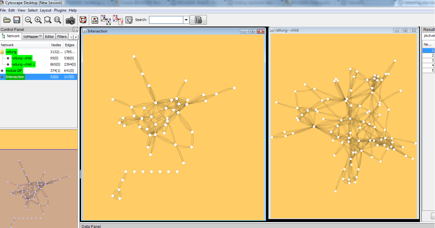
GO-ID 48731 is annotated as “system development”. This is described in GO database as “the biological process whose specific outcome is the progression of an organismal system over time, from its formation to the mature structure.” The node is relevant as it is intensely coloured and lies away from the centre of the graph. Selecting the node in BiNGO data output and clicking “Select Nodes” highlighted all nodes in the original network (not only ones in the active module) which are annotated with “system development” category. The result was a network of 865 nodes. In the Figure 5, ratlung-child is a network that was created from the active module, and ratlung-child.1 is a network that contains the genes annotated as “system development”.

Figure 5 – GO-ID 48731 in BiNGO output

Figure 6 – ‘system development” nodes in the network.

Next, the “Advanced Network Merge” plugin was used to find the intersection between those two networks.

Figure 7 – intersection between active module and nodes annotated as “system development”

GO-ID 6357

Figure 8 – GO-ID 6357 in BiNGO graphical output

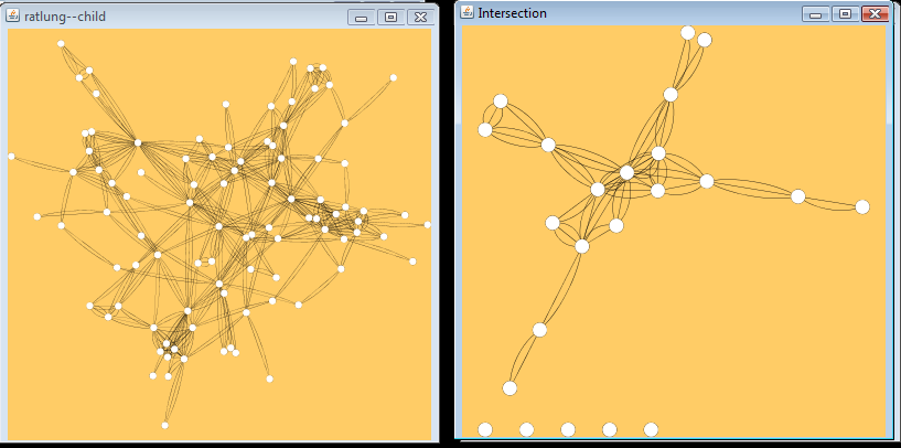
GO-ID 6357 is annotated as “regulation of transcription from RNA polymerase II promoter”. This is described as any process that modulates the frequency, rate of extent of transcription from RNA polymerase II promoter. Selecting the node in BiNGO data output and clicking “Select Nodes” resulted in a network of 292 nodes. The network was then analysed for intersecting with active module 1.

Figure 9 – Intersection between active module and nodes annotated as “regulation of transcription from RNA polymerase II promoter”

References:

S. Maere, K. Heymans and M. Kuiper, BiNGO: a Cytoscape plugin to assess overrepresentation of Gene Ontology categories in Biological Networks, Bioinformatics Applications, 21:3448 (2005)

Gene Ontology Project Website

BINGO Tutorial

by Evgeny. Also posted on my website

Adding Expression Data to the Network

Introduction

The network that I have been using is a generalised view of the interactions that may take place. By adding gene expression data to the network, I will be able to determine which interactions are 'active' under the known experimental conditions. The data provided for analysis was from an experiment to examine the changes in gene expression in the lungs of rats exposed to mustard gas (GSE1888).

The goal was to find, identify and compare the active modules and how they overlap with the network of proteins affected by mustard gas.

1. Functional Modules

When the protein interactions are represented as graphs, they can be used to investigate the functions of proteins through their interactions with neighbouring proteins. Clusters of highly interconnected proteins could not have occurred by chance and are likely to contain proteins with a common biological function (Dunn et al, 2005). Such clusters are called functional modules and their identification is a complex task.

Bader and Hogue (2003) suggested the three-stage algorithm for finding molecular complexes. The algorithm assigns weights to nodes based on “cliquishness” of a node, which is proportional to the number of nodes in the neighbourhood and inversely proportional to the vertex size of the neighbourhood.

Dunn et al. (2005) note that in certain cases, such as a prey node attached to the bait by a single edge, a poorly connected node provides useful information. Methods that use edge-betweenness, unlike many other clustering methods, will not remove such nodes and are useful when the information associated with these low degree nodes is required.

2. Finding Active Modules

The file provided for the exercise contained significance values of the difference in gene expression in rats that were exposed to 6mg/kg mustard gas for 1, 3 and 6 hours. The jActiveModules plugin was used to find active modules. The plugin identified five functional modules ranging from 69 to 95 nodes in size.

3. Examining Active Modules

Network from module 1.

1 hour: all significance values are equal to 0.999783355
3 hours: significance values in range of 4.5*10-5 to 0.489861449

Graphical view, with nodes having higher significance values coloured with darker red.

In this network, only five proteins have significance values over 0.01.

6 hours: significance values in range of 6.13*10^-8 to 0.916047284

This time, over 30 proteins have significance values over 0.01.

Network from module 2.

1 hour: all significance values are equal to 0.999783355

3 hours: significance values in range of 4.5*10^-5 to 0.489861449

6 hours: significance values in range of 6.13*10^-8 to 0.916047284

4. Comparing the Modules Identified

After networks were created from first three of the five active modules identified, the Cytoscape plugin Advanced Network Merge was used to merge these three modules.

The merged network which is coloured according to the differential expression at 6 hours was represented on the image below:

It is not immediately obvious from the picture how strongly the three networks which were merged into one overlap. One observation is that the merged network has 118 nodes, while the three child networks would have 95 + 44 + 72 = 211 nodes if there was no overlap. This is an indication that a significant number of nodes are present in two or three child networks.

Another approach may be to compare the proteins with high p-values. To fill the table below, the nodes in each of the child active modules were sorted by p-value at 6 hours. Then ten proteins with highest p-values were inserted into the table. One protein (Icam1) was present in all three “top tens”. Module 1 and 2 share one other protein (Krt19), and modules 1 and 3 share one other protein (Lpl), while modules 2 and 3 share five other proteins (Cd36, Hamp, Sacm11, Tim3, Dusp1). From this basic analysis it can be roughly estimated that all three modules are overlapped to some extent, and modules 2 and 3 are more significantly overlapped compared to module 1 and 2 or 1 and 3. Further more detailed analysis is required to make more exact conclusions.

Active Module 1	Active Module 2	Active Module 3
Lpl		Lpl
Sele
Icam1	Icam1	Icam1
Il18
Krt19	Krt19
Nr1h3
Pla2g1b
Col5a2
Nt5e
Pawr
		Axin1
	Cd36	Cd36
	Hamp	Hamp
	Sacm1l	Sacm1l
	Timp3	Timp3
		Mark3
	Dusp1	Dusp1
	Phlda1
	Pcm1
	Raf1
		Gsk3b

References:

R. Dunn, F. Dudbridge, C. Sanderson, The Use of Edge-Betweenness Clustering to Investigate Biological Function in Protein Interaction Networks, BMC Bioinformatics, 6:39 (2005)

G. Bader, C. Hogue, An automated method for finding molecular complexes in large protein interaction networks, BMC Bioinformatics, 4:2 (2003)

Feedback

You have identified and shaded active modules. However, it is more interesting at this stage to shade by fold change, rather than by significance value. By using the fold change values (1hexp, 3hexp, 6hexp) you can see which parts of your network are up/down-regulated over the course of the experiment. In the practical instructions I suggested that you use the intersection option when merging your networks. This does show you the extent of the overlap.

My Comment

It was quite stupid of me to use 'union' instead of 'intersect' when merging networks and then record that there are no obvious observations.

by Evgeny. Also posted on my website

Network Topology

Degree distribution and power law.

For a long time the graph theory modelled complex networks either as being regular objects, or as being completely random. An important finding was that the number of nodes with a given degree does not follow the Poisson distribution, but follows a power law (Barabasi & Oltvai, 2004)

That means that the probability to find a hub with a number of neighbours a magnitude higher is a magnitude lower, but still not negligible (Bode et al, 2007).

In simple terms, a node with a degree of 10 will be found 10 times less often, than the node with a degree of 1, and the node with a degree of 100 - 100 times less often.

Such networks are called scale-free, which means that it is not possible to find a typical node in the network - one that could be used to characterize the rest of the nodes. The evidence that cellular networks are scale-free came from the analysis of metabolism networks of various organisms. As a typical feature of the scale-free network, most of the proteins only participate in a few interactions, but there is a small number of proteins which participate in dozens interactions. Alternatively it can be described as a small number of hubs (highly connected nodes) which hold the whole network together. (Barabasi & Oltvai, 2004)

From the evolutionary point of view, there are two factors that explain scale-free nature of cellular networks. One is the fact that most network are a result of a very slow growth over an extended time period, and the other is that new nodes are more likely to connect to nodes which already have many links. (Barabasi & Oltvai, 2004)

Not everyone agrees to the fact that the node degree distribution follows a power law. Tanaka et al (2005) studied the two publicly available networks, the FYI (filtered yeast interactome) and human protein interaction (HPI) maps and investigated whether their node degree sequences follow a power law. Their conclusion was that usage of frequency-degree plots leads to errors which can easily be avoided by using rank-degree plots and the node degree sequences of these networks are clearly not power laws, but much closer to exponential.

Betweenness Centrality

Betweenness is a quantitative measure for describing the centrality of nodes in a network, provided as the frequency with which a node is located on the shortest path between all other nodes. Nodes with high betweenness control the flow of information across a network. There is a positive correlation between the centrality of the proteins and their essentiality in many species, and there is also a positive correlation between centrality and node degree. (Yamada & Bork, 2009)

Betweenness centrality lies at the core of both transport and structural vulnerability properties of complex networks; however, it is computationally costly, and its measurement for networks with millions of nodes is nearly impossible. (Ercsey-Ravasz & Toroczkai, 2010).

One of the practical applications of betweenness centrality is the drug design. Hormozdiari et al (2010) suggest that if the essential pathways in a pathogenic organism are known, it should be possible to compute the minimum number of proteins that need to be targeted as many essential pathways as possible. The proteins with the highest betweenness will be the most obvious choices but, of course, the algorithm is not that simple and includes a schema whether the proteins are also weighted based on the presence of an ortholog of a protein in the host. We wouldn't want a drug to target vital proteins in our own body.

Calculating and using network statistic.

Node degree distribution

It is evident that there is a large number of nodes with a low node degree, but there is only a handful of nodes with a degree over 100. The degree distribution does not appear to be random and it is known from literature that it usually follows a power law.

Figure 1 – node degree distribution in a large network.

Fitting a power law.

The power law was fitted as follows: y=3391.6 * x^-1.698. The power law explains 92.5% of the distribution, which is a very good fit. This is also evident from the fact that the residues appear to be distributed randomly to the both sides of the fitted line and close to the line.

Figure 2 – power law fitted functionFigure 3 – power law fitted graph.

Betweenness centrality

The value of betweenness centrality is normalized and therefore lies between 0 and 1.

Figure 4 – betweenness centrality in a large network.

Removing the largest component.

The largest connected component in the network being studied has 2623 nodes, which is the majority of the nodes of the whole network and the largest of the other components is only 12 nodes.

Figure 5 – largest connected components of a large network.

Below is the second largest of components, with the node marked in yellow having a high betweenness centrality of 0.7:

Figure 6 – second largest connected component of large network

This node connects two “clusters” of 5 and 4 nodes, and two other nodes. Since the definition of betweenness is “number of shortest paths from all nodes to all others that pass through that node”, it has a relatively high betweenness.

Several example nodes from the largest connected components:

A node with high betweenness centrality (0.082), high degree (150) : Cam1. The node has a high degree, so it is connected to many other nodes in the network. Therefore a significant number of shortest paths passes through the node. It can also be seen that a significant number of nodes other than Cam1 are directly connected to each other, reducing the betweenness of Cam1.

Figure 7 – Cam1 and neighbouring nodes.

A node with relatively high betweenness centrality (0.01), low degree (10) : Csnk2b. This one is not obvious to me, I would expect the betweenness of this node to be higher since it appears to be central to its five neighbours. Probably as part of the whole connected component it belongs to the peripheral area of the network.

Figure 8 – Csnk2b and neighbouring nodes.

A node with low betweenness centrality (0), relatively high degree (28) : Ndufb8. Nodes other than Ndufb8 are highly connected, so only a small number of shortest paths between nodes pass through Ndufb8.

Figure 9 – Ndufb8 and neighbouring nodes.

A node with low betweenness centrality (0), low degree (4) : Fbxo11. There is only one node here other than Fbxo11, so there are no routes between nodes other than Fbxo11 at all.

Figure 10 – Fbxo11 and neighbouring nodes.

References:

A-L Barabasi, Z. Oltvai, Network biology: Understanding the cell's functional organization, Nature Reviews Genetics, 5:101 (2004)

T. Yamada, P. Bork, Evolution of biomolecular networks - lessons from metabolic and protein interactions, Nature Reviews Molecular Cell Biology, 10:791 (2009)

R. Tanakaa, T. Yi, J. Doyle, Some protein interaction data do not exhibit power law statistics. FEBS Letters, 579:514 (2005)

C. Bode, I. Kovacs, M. Szalay, R. Palotai, T. Korcsmaros et al., Network analysis of protein dynamics, FEBS Letters, 581:2776 (2007)

M. Ercsey-Ravasz, Z. Toroczkai, Centrality scaling in large networks, Physical review letters, 105:38701(2010)

F. Hormozdiari, R. Salari, V. Bafna, S. Sahinalp, Protein-protein interaction network evaluation for identifying potential drug targets, Journal of Computational Biology, 17:669 (2010)

by Evgeny. Also posted on my website

Starting With Cytoscape

Cytoscape is a popular open source platform for visualising molecular interaction networks.

Cytoscape website

Cytoscape has a built-in plugin manager (Plugins -> Manage Plugins) which lets the user install a large number of plugins.

One of the most important applications of Cytoscape is the analysis of interaction networks. The networks are described by eXtensible Graph Markup and Modeling Language - XGMML.

XGMML

I found a sample file here

pte.xgmml

To import the file into Cytoscape, select File -> Import -> Network(multiple file types)

This is how a network typically may look.

To view all nodes and edges, apply a layout, for example Layouts -> Cytoscape Layouts -> Spring Embedded

In the Node Attribute Browser below, click "Select All Attributes". To select all nodes in the Cytoscape model, use Ctrl-A.

If the network is large, it is possible to use a selection criteria to select nodes of interes and to create a new network from the selected nodes only. For example, it is possible to sort the nodes by an attribute in the node attribute browser (or edge attribute browser), select a number of nodes and then select File -> New -> Network -> From Selected Nodes, All Edges. Cytoscape will create a child subnetwork which will only include selected nodes and/or edges.

by Evgeny. Also posted on my website