1. Introduction
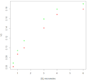
The asparatic proteinase from HIV is a target for antiviral drug design. Kuzmic et al (1996) studied the influence of mechanical stirring on the process of asparatic proteinase catalysed hydrolysis of a fluorogenic peptide. The kinetics were measured for the two reactions types, one with mechanical stirring and one without, under otherwise identical conditions. Initial velocities from both sets of reactions were plotted at initial substrate concentrations of 6, 4, 3, 1.5, 1 and 0.66 micromoles. Kuzmic et al (1996) did not include the raw data into the article, but the data was presented in Figure 1.
Figure 1. Raw data used in the exercise
For the purpose of this exercise, the raw data was visually translated from the graph into the numeric values. The data then was plotted using the following R script
conc<-c(0.66,1,1.5,3,4,6)
rate1<-c(0.0611,0.0870,0.1,0.1407,0.1685,0.1796)
rate2<-c(0.0685,0.0944,0.1148,0.1592,0.1796,0.1907)

plot(conc,rate1,ylim=range(c(rate1,rate2)),lwd=2,col="red",xlab="[S], micromoles",ylab="V0")
par(new=TRUE)
plot(conc,rate2,ylim=range(c(rate1,rate2)),lwd=2,col="green",axes=FALSE,xlab="",ylab="")
Figure 2. Raw data plotted with R
2. Using the Lineweaver-Burk plot
Next, the reciprocal values were produced and the Lineweaver-Burk plot was constructed and plotted using the following R script
concLB<-1/conc
rate1LB<-1/rate1
rate2LB<-1/rate2
plot(concLB,rate1LB,ylim=range(c(rate1LB,rate2LB)),lwd=2,col="red",xlab="1/[S]",ylab="1/V0")
par(new=TRUE)
plot(concLB,rate2LB,ylim=range(c(rate1LB,rate2LB)),lwd=2,col="green",xlab="",ylab="")
Figure 3. Lineweaver-Burk plot with R
Next, the least squares regression was applied to the plot of reciprocals to establish the values of Km and Vmax
fit<-lm(rate1LB~concLB)
fit

Call:
lm(formula = rate1LB ~ concLB)

Coefficients:
(Intercept)       concLB
      4.050        7.626
From the results of the script, the regression line for the data gathered in the absence of stirring is described by the following equation
1/ Vmax = 4.050 + 7.626*(1/ Km)
Vmax = 1/4.050 = 0.2469
-7.626*(1/ Km) = 4.050
-(1/ Km)=0.5311
Km = 1.8829
Similarly, the following script was applied to the second set of data
fit<-lm(rate2LB~concLB)
fit

Call:
lm(formula = rate2LB ~ concLB)

Coefficients:
(Intercept)       concLB
      3.957        6.932
Call:
lm(formula = rate2LB ~ concLB)

Coefficients:
(Intercept)       concLB
      4.166        7.170
The regression line was described by the following equation.
1/ Vmax = 4.166 + 7.170*(1/ Km), from which
Vmax = 0.24, Km = 1.7212
3. Using the Hanes-Woolf plot
The Lineweaver-Burk plot is prone to errors as small errors in reaction rate measurement increase the reciprocal. Among alternative linear forms is the Hanes-Woolf plot where the ratio of the substrate concentration to the reaction velocity is plotted against substrate concentration. The data was used to plot the Hanes-Woolf plot using the following R script
rate1HW<-conc/rate1
rate2HW<-conc/rate2
plot(conc,rate1HW,ylim=range(c(rate1HW,rate2HW)),lwd=2,col="red",xlab="[S]",ylab="[S]/V0")
par(new=TRUE)
plot(conc,rate2HW,ylim=range(c(rate1HW,rate2HW)),lwd=2,col="green",xlab="",ylab="")
The least squares regression was applied
fit<-lm(rate1HW~conc)
fit

Call:
lm(formula = rate1HW ~ conc)

Coefficients:
(Intercept)         conc
      8.005        4.191
The regression line is described by the following equation
(S/v) = 8.005 + 4.191*S
Km = 8.005/4.191 = 1.91
Km / Vmax = 8.005
Vmax = 1.91/8.005 = 0.2386
Similar script was used to process the data taken in the presence of stirring.
fit<-lm(rate2HW~conc)
fit

Call:
lm(formula = rate2HW ~ conc)

Coefficients:
(Intercept)         conc
      6.726        4.054
The regression line is described by the following equation
(S/v) = 6.726 + 4.054*S
Km = 1.659, Vmax = 0.2467
4. Using the R language package
Finally, the non-linear self-starting Michaelis-Menten model, which is part of the R language, was used to estimate the values of Vmax and Km in the absence of stirring using the following R script
model<nls(rate1~SSmicmen(conc,a,b))
summary(model)

and providing the following output

Formula: rate1 ~ SSmicmen(conc, a, b)

Parameters:
  Estimate Std. Error t value Pr(>|t|)
a  0.23953    0.01188  20.166 3.57e-05 ***
b  1.92898    0.23804   8.104  0.00126 **
---
Signif. codes:  0 *** 0.001 ** 0.01 * 0.05 . 0.1   1

Residual standard error: 0.005621 on 4 degrees of freedom

Number of iterations to convergence: 0
Achieved convergence tolerance: 1.244e-06
Which estimated Vmax = 0.23953 and Km =1.92898
Similar results for the reaction with stirring were
model<-nls(rate2~SSmicmen(conc,a,b))
summary(model)

Formula: rate2 ~ SSmicmen(conc, a, b)

Parameters:
  Estimate Std. Error t value Pr(>|t|)
a 0.248409   0.006281   39.55 2.44e-06 ***
b 1.682884   0.111784   15.05 0.000113 ***
---
Signif. codes:  0 *** 0.001 ** 0.01 * 0.05 . 0.1   1

Residual standard error: 0.003319 on 4 degrees of freedom

Number of iterations to convergence: 0
Achieved convergence tolerance: 2.261e-06
Which estimated Vmax = 0.248409 and Km =1.682884
5. Conclusion
For reference, Kuzmic et al (1996) estimated the best-fit values of kinetic constants as Km (1.71 ± 0.28) μM, and Vmax (0.235 ± 0.015) abstract units/s in the absence of stirring, and Km (2.31 ± 0.24) μM, and Vmax (0.279 ± 0.012) with stirring. The results obtained by different methods were summarised in Table 1.
| L-B Plot | H-W Plot | SSmicmen | Kuzmic et al | |
|---|---|---|---|---|
| No Stirring, Km, μM | 1.8829 | 1.91 | 1.92898 | 1.71 ± 0.28 |
| No Stirring, Vmax | 0.2469 | 0.2386 | 0.23953 | 0.235 ± 0.015 |
| Stirring, Km, μM | 1.7212 | 1.659 | 1.682884 | 2.31 ± 0.24 |
| Stirring, Vmax | 0.24 | 0.2467 | 0.248409 | 0.279 ± 0.012 |
Table 1. Michaelis-Menten parameters estimated by various methods
References:
Crawley, M, The R Book, Wiley, 2007
Kuzmic P, Peranteau A, Garcia-Echeverria C, Rich D, Mechanical Effects on the Kinetics of the HIV Proteinase Deactivation, Biochemical and Biophysical Research Communications 221, 313-317 (1996)
by Evgeny. Also posted on my website


