1. Bayesian Inference
Bayesian rule is a mathematical rule that explains how the estimate of the probability changes as new evidence is collected. It relates the odds of event A1 to event A2 before and after conditioning on event B (1).
As an example, assume that there is a bag containing black and white balls, but the percentage of colours is unknown. As more and more balls are drawn from the bag, the probability of the next ball being white (or black) can be calculated with higher precision. In this case, A1 is the probability of white ball being drawn, A2 of the black ball, and B is the set of the balls already drawn, such as “of 10 balls 4 were black and 6 were white”.
Frequentist approach to Bayes’ rule is to consider probabilities of A1 and A2 as known and fixed, while in Bayesian they are considered random variables. Bayesian approach also considers prior probability, or just the prior, which expresses uncertainty before the data is taken into account. It makes possible to introduce subjective knowledge of the problem into the model in the form of prior information. Among the drawbacks of the approach is the need to evaluate multi-dimensional integrals numerically, which gets worse as the number of parameters in the system increases. Introduction of conjugate prior is an attempt to solve these drawbacks. Conjugate prior is such prior distribution that the prior and posterior are in the same family of distributions. Markov Chains are useful because under certain conditions, a memoryless process can be generated which has the same limiting distribution as the random variable that the calculation is trying to simulate.
2. Markov Chains
A Markov chain is a process which can be in a number of states. The process starts in one of the states and moves successively from one to another. Each move is called a step. At each step a process has a probability to move to another state, and the probability does not depend on any of the previous states of the process. That is why such process is called “memoryless”.
Example: In a weather model, a day can be either nice, rainy or snowy. If the day is nice, the next day will be either rainy or snowy with 50% probability. If the day is rainy or snowy, it will stay the same with 50% probability, or will change to one of the other two possibilities with 25% probability. This is a Markov chain because the process determines its next state base on the current state only, without any prior information. The probabilities can be presented in the transition matrix (2).

The first row presents the probabilities of the next day’s weather if today is rainy (R): ½ that it will remain rainy, ¼ that it will be nice and ¼ that it will be snowy. The sum of probabilities across the row must be equal to 1.
3. Monte Carlo Methods
Markov Chains Monte Carlo (MCMC) methods are computational algorithms which randomly sample from the process. The aim of the methods is to estimate something that is too difficult or time consuming to find deterministically. Using the example above, assume that the probabilities in the matrix are not known. A MCMC could simulate a thousand rainy days and count the number of snowy, rainy and nice days that follow. The same could be repeated for snowy and nice days.
The original Monte Carlo approach was developed to use random number generation to compute integrals. If a complex integral can be decomposed into a function f(x) and a probability density function p(x), then the integral can be expressed as an expectation of f(x) over the density p(x) (3)

Now, if we draw a large number of x1, ..., xn of random variables from the density p(x), then we end up with (4), which is referred to as Monte Carlo integration.

3.1. Markov Chain Convergence
It can be shown that if matrix P is the transition matrix for a Markov chain and pij element is the probability of transitioning from state i to state j, then the element pij(n) of the matrix Pn gives the probability that the Markov chain starting in state si will be in state sj after n steps. Using the transitional matrix (2), on the sixth step of multiplying the matrix by itself the following state will be reached (5). Such Markov chain is called regular (not all Markov chains are regular). The long-range predictions for this chain are independent of the starting state.

Continuing the example, assume that the initial probabilities for the weather conditions on the starting day of the chain are equal. This will be called a probability vector, which in the example will be as shown in (6).
It can be shown that the probability of the chain being in the state si after n steps is the ith entry in the vector (7).
If, as in the example, the chain is regular, it will converge to a stationary distribution, when the probability of the chain being in state i is independent of the initial distribution. In the weather example, the stationary distribution is shown in (8).
3.2. Ergodicity and Reversibility
If the process that starts from state i will ever re-enter state i, such state is called recurrent. Additionally, such state is called nonnull if it re-enters state i in n steps, where n is finite. A process is called aperiodic if the greatest common divisor of return steps to any state is 1. For example, if the chain re-enters a state after 2, 4, 6 steps and so on, such chain is not aperiodic. A process is called irreducible if any state can be reached from any other state in a finite number of moves. A chain that is recurrent nonnull, aperiodic and irreducible is called ergodic, and the ergodic theorem states that a unique limiting distribution exists for the chain and such distribution is independent of initial distribution.
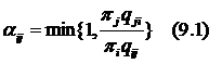
A Markov chain is reversible if (9) is satisfied for all i, j, where u is the stationary distribution and pij are elements of the transition matrix.
Ergodicity and reversibility are the two principles behind the Metropolis-Hastings algorithms.
3.3. Metropolis-Hastings algorithms
One of the problems of applying Monte Carlo integration is in obtaining samples from some complex probability distribution. Mathematical physicists attempted to integrate complex functions by random sampling. Metropolis showed how to construct the desired transition matrix and later Hastings generalized the algorithm. The essential idea of the algorithm is to construct a reversible Markov chain for given distribution π such, that its stationary distribution is π. It starts with generating the candidate j from a proposal transition matrix Q. This matrix Q transitions from current state i to proposal j. Proposal j is then accepted with some probability αij. If the rejection takes place, then the next state retains the current value. The summary of the algorithm is as follows:
- Start with arbitrary X0. Then, at each iteration t = 1, ..., N:
- Sample j~qij. Q={qij} is the transition matrix.
- Generate u – a uniformly distributed random number between 0 and 1.
- With probability (9.1), if u <= αij, set Xt+1 = j, else set Xt+1 = i.
Such algorithm randomly attempts to move about the sample space, sometimes accepting the transitions and sometimes remaining in the same state. Acceptance ratio indicates how probable the proposed sample is in respect to the current sample. If the next state is more probable than the current, the transition is always accepted. If the next step is less probable, it will be occasionally accepted, but more often rejected. Intuitively, this is why this algorithm works, tending to stay away from the regions with low-density and mostly remaining in the high-density regions.
A key issue in the successful implementation of the algorithm is the number of steps until the chain approaches stationarity, which is called the burn-in period. Typically first 1000 to 5000 elements are thrown out and then a test is used to assess whether stationarity has been reached.
3.4. Gibbs Sampling
Gibbs sampling is a special case of Metropolis-Hastings sampling where the random value is always accepted. The key is the fact that only distributions where all random variables but one are assigned fixed values are considered. The benefit is that such distributions are much easier to simulate compared to complex joint distributions. Instead of generating a single n-dimensional vector in a single pass, n random variables are simulated sequentially from the n conditionals.
A Gibbs stopper is an approach to convergence based on comparing the Gibbs sampler and the target distribution. Weights are plotted as a function of the sampler iteration number. As the sampler approaches stationarity, the distribution of weights is expected to spike.
4. Example
4.1. Initial Data
Table 1 contains the field goal shooting record of LeBron James for the seasons 2003 to 2009. The goal of the simulation was to use OpenBUGS to carry out a MCMC Bayesian simulation and produce a posterior distribution to the probability of the player’s shooting success.

Table 1 – LeBron James Goal Shooting Record
4.2. The Model
The model for the success probabilities of LeBron James is given by (10)
where k = 2, ..., 7, corresponding to seasons from 2004/5 to 2009/10, and π1 is estimated individually as a success probability for 2003/4 season. Rk are performances for the current seasons. A beta prior is the success probability for the first season and gamma priors are relative successes Rk.
Likelihood for this model is given by (11).

The likelihood is written in OpenBUGS as
for (k in 1:YEARS){ y[k] ~ dbin( pi[k], N[k] ) }while the model for success probabilities is expressed as follows:
for (k in 2:YEARS){ pi[k]<-pi[k-1]*R[k] }The data for the model specifies the values of the successes and total attempts (yi and Ni) for each season. Initial values for the model must be specified for π1 and Rk as follows:
list(pi=c(0.5, NA, NA, NA, NA, NA, NA), R=c(NA, 1,1,1,1,1,1))
No initial values were specified for π2 ... π7 since they are deterministic and for R1 since it is constant. Actual initial data used for the model is attached as separate initX.txt files, where X is the number of the chain.
4.3. One Chain Calculation
The initial calculation was run with 1000 samples burn-in and 2000 sample points, for one chain. The posterior summaries were presented in Figure 1

Figure 1 – Posterior summaries for one chain calculation
From these results, the expected success rates for James LeBron was 42.24% for the season of 2003/4, increased by a factor of 1.1 for the season of 2004/5, then stayed close to the level of 2003/4 season for the next 2 seasons (posterior means for R3 = 1.036 and R4 = 0.9863) and then was increasing steadily for the next 3 seasons.
Since Ri indicates the relative performance of a current season in comparison to the previous one, it can be reported that the player was steadily increasing his performance over the duration of the seven season, with one especially significant increase of 10.5% early in the career.
Further, posterior distributions of the relative performance vector R were analysed by using the Inference -> Compare function and producing the boxplot, which is presented in Figure 2.

Figure 2 – The boxplot of R
The limits of boxes represent the posterior quartiles and the middle bar – the posterior mean. The endings of the whisker lines are 2.5% and 97.5% posterior percentiles.
Posterior density can be estimated by plotting the success rate density for a season. Figure 3 represents the posterior density for each season (πi)

Figure 3 – Posterior density for each season
Checking convergence is not a straightforward task. While it is usually easy to say when the convergence definitely was not reached, it is difficult to conclusively say if the chain has converged. Convergence can be checked by using the trace option from Inference -> Samples menu. Figure 4 represents the history plots for πi.

Figure 4 – History Plots for πi, one chain
It is clear that π7 has converged, while the result for other seasons is not so obvious. Multiple chain calculation with a higher number of iterations may be helpful. Another reason to use the higher number of iterations is the reduction of Monte Carlo error in case it is too high – it decreases as the number of iteration grows. In fact, the value of Monte Carlo error can be used to decide when to stop simulation.
4.4. Multiple chain calculation
The main difference between the single and multiple chain calculations is the fact that a separate set of initial values is required for each chain. The following initial values were used for the three chains:
list(pi=c(0.5, NA, NA, NA, NA, NA, NA), R=c(NA, 1,1,1,1,1,1))
list(pi=c(0.9, NA, NA, NA, NA, NA, NA), R=c(NA, 1,1,1,1,1,1))
list(pi=c(0.1, NA, NA, NA, NA, NA, NA), R=c(NA, 1,1,1,1,1,1))
The posterior statistics for this calculation were presented in Figure 5.

Figure 5 – Posterior summaries for multiple chain calculation
The trace plots now contain one line for each chain. The history plots for πi for this calculation were presented in Figure 6.

Figure 6 – History Plots for πi, multiple chains
References
Ntzoufras I, Bayesian Modeling Using WinBUGS, 2009, Wiley, England
Reich B, Hodges J, Carlin B, Reich A, A Spatial Analysis of Basketball Shot Chart Data, 2005, NSCU Statistics
Walsh B, Markov Chain Monte Carlo and Gibbs Sampling, 2004, MIT Lecture Notes
Mathematics for Metabolic Modelling - Course Materials 2012, University of Manchester, UK
by Evgeny. Also posted on my website